Page 377 - Introduction to Statistical Pattern Recognition

7 Nonparametric Classification and Error Estimation 359

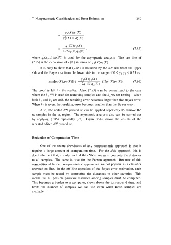
(7.85)

where qi(X,,) Eqj(X) is used for the asymptotic analysis. The last line of
(7.85) is the expression of r(X) in terms of 4 I(X)q2(X).
It is easy to show that (7.85) is bounded by the NN risk from the upper
side and the Bayes risk from the lower side in the range of 0 I 4 I q2 I 0.25 as

The proof is left for the reader. Also, (7.85) can be generalized to the case
where the k I NN is used for removing samples and the k2NN for testing. When
both kl and k2 are odd, the resulting error becomes larger than the Bayes error.
When k2 is even, the resulting error becomes smaller than the Bayes error.
Also, the edited NN procedure can be applied repeatedly to remove the
o,-samples in the o,-region. The asymptotic analysis also can be carried out
by applying (7.85) repeatedly [22]. Figure 7-16 shows the results of the
repeated edited NN procedure.

Reduction of Computation Time

One of the severe drawbacks of any nonparametric approach is that it
requires a large amount of computation time. For the kNN approach, this is
due to the fact that, in order to find the kNN’s, we must compute the distances
to all samples. The same is true for the Parzen approach. Because of this
computational burden, nonparametric approaches are not popular as a classifier
operated on-line. In the off-line operation of the Bayes error estimation, each
sample must be tested by computing the distances to other samples. This
means that all possible pairwise distances among samples must be computed.
This becomes a burden to a computer, slows down the turn-around time, and
limits the number of samples we can use even when more samples are
available.