Page 374 - Introduction to Statistical Pattern Recognition

356 Introduction to Statistical Pattern Recognition

perty will be true regardless of the underlying distribution. Table 7-6 shows
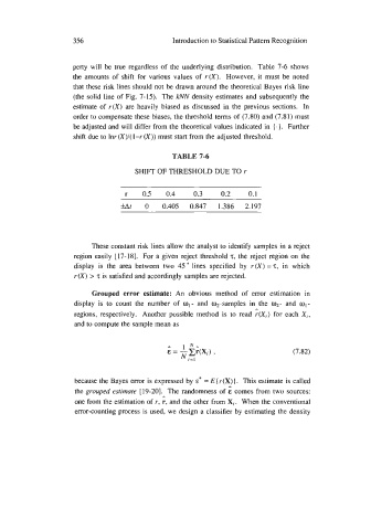
the amounts of shift for various values of r(X). However, it must be noted
that these risk lines should not be drawn around the theoretical Bayes risk line
(the solid line of Fig. 7-15). The kNN density estimates and subsequently the
estimate of r(X) are heavily biased as discussed in the previous sections. In
order to compensate these biases, the threshold terms of (7.80) and (7.81) must
be adjusted and will differ from the theoretical values indicated in (. ). Further
shift due to lnr (X)l( 1-r (X)) must start from the adjusted threshold.

TABLE 7-6

SHIFT OF THRESHOLD DUE TO r

r 0.5 0.4 0.3 0.2 0.1

kAt 0 0.405 0.847 1.386 2.197

These constant risk lines allow the analyst to identify samples in a reject
region easily [17-181. For a given reject threshold z, the reject region on the
display is the area between two 45 lines specified by r(X) = 2, in which
r(X) > z is satisfied and accordingly samples are rejected.

Grouped error estimate: An obvious method of error estimation in
display is to count the number of ol- and w2-samples in the 02- and wI-
A
regions, respectively. Another possible method is to read r(Xj) for each Xi,
and to compute the sample mean as

(7.82)

because the Bayes error is expressed by E* = E(r(X)]. This estimate is called
the grouped estimate [19-201. The randomness of E comes from two sources:
A
one from the estimation of r, r, and the other from Xi. When the conventional
error-counting process is used, we design a classifier by estimating the density