Page 108 - Petroleum Production Engineering, A Computer-Assisted Approach

Guo, Boyun / Computer Assited Petroleum Production Engg 0750682701_chap08 Final Proof page 100 20.12.2006 10:36am

8/100 PETROLEUM PRODUCTION ENGINEERING FUNDAMENTALS
8.5 Model Identification
Rate at End of Year Yearly Production
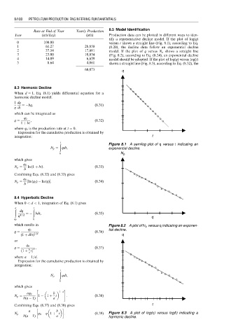
Year (stb/day) (stb) Production data can be plotted in different ways to iden-
tify a representative decline model. If the plot of log(q)
0 100.00 — versus t shows a straight line (Fig. 8.1), according to Eq.
1 61.27 28,858 (8.20), the decline data follow an exponential decline
2 37.54 17,681 model. If the plot of q versus N p shows a straight line
3 23.00 10,834 (Fig. 8.2), according to Eq. (8.24), an exponential decline
4 14.09 6,639 model should be adopted. If the plot of log(q) versus log(t)
5 8.64 4,061 shows a straight line (Fig. 8.3), according to Eq. (8.32), the
68,073 q

8.3 Harmonic Decline
When d ¼ 1, Eq. (8.1) yields differential equation for a
harmonic decline model:
1 dq
¼ bq, (8:31)
q dt
which can be integrated as
q 0
q ¼ , (8:32)
1 þ bt
where q 0 is the production rate at t ¼ 0.
Expression for the cumulative production is obtained by
integration: t
ð t Figure 8.1 A semilog plot of q versus t indicating an
N p ¼ qdt, exponential decline.
0 N p
which gives
q 0
N p ¼ ln (1 þ bt): (8:33)
b
Combining Eqs. (8.32) and (8.33) gives
q 0
N p ¼ ½ ln (q 0 ) ln (q)Š: (8:34)
b

8.4 Hyperbolic Decline
When 0 < d < 1, integration of Eq. (8.1) gives
ð q ð t
dq
¼ bdt, (8:35)
q 1þd q
q 0 0
which results in Figure 8.2 A plot of N p versus q indicating an exponen-
q 0 tial decline.
q ¼ (8:36)
(1 þ dbt) 1=d q
or
q 0
q ¼ a , (8:37)
b
1 þ t
a
where a ¼ 1=d.
Expression for the cumulative production is obtained by
integration:
ð t
N p ¼ qdt,
0
which gives
" 1 a #
aq 0 b
N p ¼ 1 1 þ t : (8:38)
b(a 1) a
Combining Eqs. (8.37) and (8.38) gives t

a b
N p ¼ q 0 q 1 þ t : (8:39) Figure 8.3 A plot of log(q) versus log(t) indicating a
b(a 1) a harmonic decline.