Page 111 - Petroleum Production Engineering, A Computer-Assisted Approach

Guo, Boyun / Computer Assited Petroleum Production Engg 0750682701_chap08 Final Proof page 103 20.12.2006 10:36am

PRODUCTION DECLINE ANALYSIS 8/103
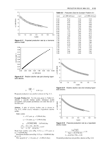
12 Table 8.3 Production Data for Example Problem 8.4
10 t (yr) q (1,000 stb/day) t (yr) q (1,000 stb/day)
q (1,000 Stb/d) 8 6 0.20 9.28 2.20 5.05
2.10
9.63
5.18
0.10
2.30
4.92
8.95
0.30
2.40
0.40
8.64
4.80
0.50
4
0.60 8.35 2.50 4.68
8.07
4.57
2.60
2 0.70 7.81 2.70 4.46
0.80 7.55 2.80 4.35
0 0.90 7.32 2.90 4.25
0.0 1.0 2.0 3.0 4.0 5.0 6.0 1.00 7.09 3.00 4.15
t (year) 1.10 6.87 3.10 4.06
1.20 6.67 3.20 3.97
Figure 8.11 Projected production rate by a harmonic 1.30 6.47 3.30 3.88
decline model. 1.40 6.28 3.40 3.80
1.50 6.10 3.50 3.71
1.60 5.93 3.60 3.64
0.38 1.70 5.77 3.70 3.56
0.36 1.80 5.61 3.80 3.49
1.90 5.46 3.90 3.41
0.34 2.00 5.32 4.00 3.34
−∆q/∆t/q (year −1 ) 0.30 12
0.32
0.28
0.26
0.24 10
0.22 8
0.20
3.00 4.00 5.00 6.00 7.00 8.00 9.00 10.00 q (1,000 stb/d) 6
q (1,000 stb/d) 4
Figure 8.12 Relative decline rate plot showing hyper- 2
bolic decline.
0
0.0 1.0 2.0 3.0 4.0 5.0
t (year)
Figure 8.13 Relative decline rate shot showing hyper-
10;000 1
b ¼ 5;680 ¼ 0:38 1=yr: bolic decline.
2
Projected production rate profile is shown in Fig. 8.11.
12
Example Problem 8.4 For the data given in Table 8.3, 10
identify a suitable decline model, determine model
parameters, and project production rate until the end of 8
the fifth year.
Solution A plot of relative decline rate is shown in q (1,000 stb/d) 6
Fig. 8.12, which clearly indicates a hyperbolic decline 4
model.
2
Select points
t 1 ¼ 0:2 year, q 1 ¼ 9,280 stb=day 0
0.0 1.0 2.0 0.3 4.0 5.0 6.0
t 2 ¼ 3:8 years, q 2 ¼ 3,490 stb=day t (year)
p ffiffiffiffiffiffiffiffiffiffiffiffiffiffiffiffiffiffiffiffiffiffiffiffiffiffiffiffiffi
q 3 ¼ (9,280)(3,490) ¼ 5,670 stb=day Figure 8.14 Projected production rate by a hyperbolic
decline model.
b 0:2 þ 3:8 2(1:75)
¼ ¼ 0:217
a (1:75) (0:2)(3:8)
2
log 10,000
Read from decline curve (Fig. 8.13) t 3 ¼ 1:75 years at 6,280
q 3 ¼ 5,670 stb=day. a ¼ log (1 þ (0:217)(1:4) ) ¼ 1:75
Read from decline curve (Fig. 8.13) q 0 ¼ 10,000 stb=day b ¼ (0:217)(1:758) ¼ 0:38
at t 0 ¼ 0.

Pick up point (t ¼ 1:4 years, q ¼ 6,280 stb=day). Projected production rate profile is shown in Fig. 8.14.