Page 116 - Petroleum Production Engineering, A Computer-Assisted Approach

Guo, Boyun / Computer Assited Petroleum Production Engg 0750682701_chap09 Final Proof page 110 21.12.2006 2:16pm

9/110 EQUIPMENT DESIGN AND SELECTION
9.1 Introduction
Most oil wells produce reservoir fluids through tubing
strings. This is mainly because tubing strings provide
good sealing performance and allow the use of gas expan-
sion to lift oil. Gas wells produce gas through tubing Stress (s)
strings to reduce liquid loading problems.
Tubing strings are designed considering tension, col-
lapse, and burst loads under various well operating condi-
tions to prevent loss of tubing string integrity including
mechanical failure and deformation due to excessive
stresses and buckling. This chapter presents properties of Strain (e)
the American Petroleum Institute (API) tubing and special
considerations in designing tubing strings.
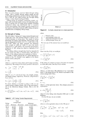
Figure 9.1 A simple uniaxial test of a metal specimen.
where
9.2 Strength of Tubing
The API defines ‘‘tubing size’’ using nominal diameter and n ¼ Poison’s ratio
weight (per foot). The nominal diameter is based on the s 1 ¼ axial principal stress, psi
internal diameter of tubing body. The weight of tubing s 2 ¼ tangential principal stress, psi
determines the tubing outer diameter. Steel grades of tub- s 3 ¼ radial principal stress, psi.
ing are designated to H-40, J-55, C-75, L-80, N-80, C-90, For our case of the uniaxial test, we would have
and P-105, where the digits represent the minimum
yield strength in 1,000 psi. Table 9.1 gives the tensile s 1 ¼ s
requirements of API tubing. The minimum performance s 2 ¼ 0 : (9:5)
properties of API tubing are listed in Appendix B of
this book. s 3 ¼ 0
The tubing collapse strength data listed in Appendix B Then from Eq. (9.4), we would get
do not reflect the effect of biaxial stress. The effect of
tension of the collapse resistance is analyzed as follows. 1 1 þ v 2 2
Consider a simple uniaxial test of a metal specimen as U ¼ 2 3E s þ s
shown in Fig. 9.1, Hooke’s Law applies to the elastic
portion before yield point: U ¼ 1 þ v s : (9:6)
2
3E
s ¼ E«, (9:1)
where s, «, and E are stress, strain, and Young’s modulus, If the failure of a material is taken to be when the material
respectively. The energy in the elastic portion of the test is is at the yield point, then Eq. (9.6) is written

1 1 P Dl 1 (P Dl) 1 þ v 2
U u ¼ s« ¼ ¼ U f ¼ s , (9:7)
y
2 2 A L 2 V 3E
1 W where s y is yield stress. The definition of an ‘‘equivalent
U u ¼ , (9:2) stress’’ is the energy level in 3D, which is equivalent to the
2 V
criteria energy level. Thus,
where P, A, L, V, and Dl are force, area, length, volume,
and length change, respectively. However, using Hooke’s 1 þ v 2 1 þ v 2
Law, we have 3E s ¼ 3E s y
e

1 1 s 1 s 2 and
U u ¼ s« ¼ s ¼ : (9:3)
2 2 E 2 E
s e ¼ s y , (9:8)
To assess whether a material is going to fail, we use
various material failure criteria. One of the most import- where s e is the equivalent stress. The collapse pressure is
ant is the Distortion Energy Criteria. This is for 3D expressed as
and is " #
D 1
1 1þv p c ¼ 2s y t , (9:9)
2
2
2
ð
ð
U ¼ ½ s 1 s 2 Þ þ s 2 s 3 Þ þ s 3 s 1 Þ Š, (9:4) D 2
ð
2 3E t
where D is the tubing outer diameter (OD) and t is wall
thickness.
For the 3D case, we can consider
Table 9.1 API Tubing Tensile Requirements
1 þ v 2
Yield U ¼ 3E s , (9:10)
e
strength (psi)
Tubing Minimum where s e is the equivalent stress for the 3D case of
grade Minimum Maximum tensile strength (psi)

H-40 40,000 80,000 60,000 1 þ v s ¼ 1 1 þ v (s 1 s 2 ) þ (s 2 s 3 ) 2
2
2
J-55 55,000 80,000 75,000 3E e 2 3E

C-75 75,000 90,000 95,000 þ (s 3 s 1 ) ; (9:11)
2
L-80 80,000 95,000 95,000
N-80 80,000 110,000 100,000 thus,
C-90 90,000 105,000 100,000 1 n o
2
2
2
ð
P-105 105,000 135,000 120,000 s ¼ 2 ð s 1 s 2 Þ þ s 2 s 3 Þ þðs 3 s 1 Þ 2 : (9:12)
e