Page 109 - Petroleum Production Engineering, A Computer-Assisted Approach

Guo, Boyun / Computer Assited Petroleum Production Engg 0750682701_chap08 Final Proof page 101 20.12.2006 10:36am

PRODUCTION DECLINE ANALYSIS 8/101
decline data follow a harmonic decline model. If the plot of decline model may be verified by plotting the relative
N p versus log(q) shows a straight line (Fig. 8.4), according decline rate defined by Eq. (8.1). Figure 8.5 shows such a
to Eq. (8.34), the harmonic decline model should be used. plot. This work can be easily performed with computer
If no straight line is seen in these plots, the hyperbolic program UcomS.exe.

8.6 Determination of Model Parameters
N p
Once a decline model is identified, the model parameters a
and b can be determined by fitting the data to the selected
model. For the exponential decline model, the b value can
be estimated on the basis of the slope of the straight line in
the plot of log(q) versus t (Eq. [8.23]). The b value can also
be determined based on the slope of the straight line in the
plot of q versus N p (Eq. [8.27]).
For the harmonic decline model, the b value can be
estimated on the basis of the slope of the straight line in
the plot of log(q) versus log(t) or Eq. (8.32):
q 0
1
b ¼ q 1 : (8:40)
t 1
The b value can also be estimated based on the slope of the
straight line in the plot of N p versus log(q) (Eq. [8.34]).
q For the hyperbolic decline model, determination of a
and b values is somewhat tedious. The procedure is shown
Figure 8.4 A plot of N p versus log(q) indicating a har- in Fig. 8.6.
monic decline. Computer program UcomS.exe can be used for both
model identification and model parameter determination,
− ∆q as well as production rate prediction.
q∆t
Harmonic decline
Hyperbolic decline 8.7 Illustrative Examples
Example Problem 8.2 For the data given in Table 8.1,
identify a suitable decline model, determine model
parameters, and project production rate until a marginal
Exponential decline rate of 25 stb/day is reached.

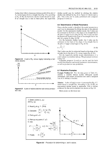
Solution A plot of log(q) versus t is presented in Fig. 8.7,
q which shows a straight line. According to Eq. (8.20), the
exponential decline model is applicable. This is further
Figure 8.5 A plot of relative decline rate versus produc- evidenced by the relative decline rate shown in Fig. 8.8.
tion rate. Select points on the trend line:

1. Select points (t , q )
1
1
and (t 2 , q 2 )
at q = q q
2. Read t 3 3 1 2
q
b t + t − 2t 3
1
2
3. Calculate =
2
a t − t t
1 2
3
4. Find q 0 at t = 0 1
5. Pick up any point (t*, q*) q
6. Use q 3 (t*, q* )
log 0 2
q q *
q * = 0 a a =
1+ b t * log 1+ b t *
a a
t 3
b
7. Finally b = a t
a
Figure 8.6 Procedure for determining a- and b-values.