Page 110 - Petroleum Production Engineering, A Computer-Assisted Approach

Guo, Boyun / Computer Assited Petroleum Production Engg 0750682701_chap08 Final Proof page 102 20.12.2006 10:36am

8/102 PETROLEUM PRODUCTION ENGINEERING FUNDAMENTALS
10,000 t 1 ¼ 5 months, q 1 ¼ 607 stb=day
t 2 ¼ 20 months, q 2 ¼ 135 stb=day
1,000 Decline rate is calculated with Eq. (8.23):
135
1
q (STB/D) 100 Projected production rate profile is shown in Fig. 8.9.
b ¼
ln
¼ 0:11=month
607
(5 20)
10 0.40
0.35
1
0 5 10 15 20 25 30
−∆q/∆t/q (year −1 )
t (month) 0.30
Figure 8.7 A plot of log(q) versus t showing an expo- 0.25
nential decline. 0.20

Table 8.1 Production Data for Example Problem 8.2
0.15
t (mo) q (stb/day) t (mo) q (stb/day)
0.10
1.00 904.84 13.00 272.53 3.00 4.00 5.00 6.00 7.00 8.00 9.00 10.00
2.00 818.73 14.00 246.60 q (1000 stb/d)
3.00 740.82 15.00 223.13
4.00 670.32 16.00 201.90 Figure 8.10 Relative decline rate plot showing har-
5.00 606.53 17.00 182.68 monic decline.
6.00 548.81 18.00 165.30
7.00 496.59 19.00 149.57
8.00 449.33 20.00 135.34
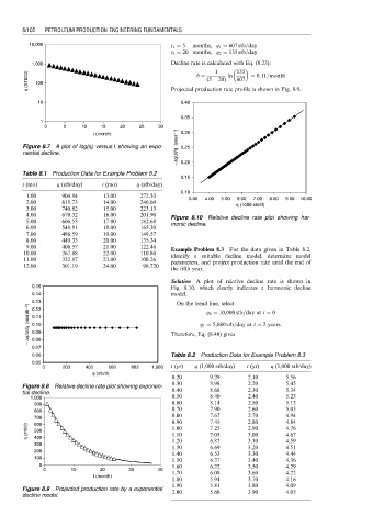
9.00 406.57 21.00 122.46 Example Problem 8.3 For the data given in Table 8.2,
10.00 367.88 22.00 110.80 identify a suitable decline model, determine model
11.00 332.87 23.00 100.26 parameters, and project production rate until the end of
12.00 301.19 24.00 90.720
the fifth year.
Solution A plot of relative decline rate is shown in
0.15 Fig. 8.10, which clearly indicates a harmonic decline
0.14 model.
0.13 On the trend line, select
− ∆q/∆t/q (month −1 ) 0.11 Therefore, Eq. (8.40) gives
0.12
q 0 ¼ 10,000 stb=day at t ¼ 0
q 1 ¼ 5,680 stb=day at t ¼ 2 years:
0.10
0.09
0.08
0.07
0.06 Table 8.2 Production Data for Example Problem 8.3
0.05
3 203 403 603 803 1,003 t (yr) q (1,000 stb/day) t (yr) q (1,000 stb/day)
q (stb/d)
0.20 9.29 2.10 5.56
0.30 8.98 2.20 5.45
Figure 8.8 Relative decline rate plot showing exponen-
tial decline. 0.40 8.68 2.30 5.34
1,000 0.50 8.40 2.40 5.23
900 0.60 8.14 2.50 5.13
800 0.70 7.90 2.60 5.03
700 0.80 7.67 2.70 4.94
0.90 7.45 2.80 4.84
600
q (stb/d) 500 1.00 7.25 2.90 4.76
4.67
1.10
3.00
7.05
400
300 1.20 6.87 3.10 4.59
1.30 6.69 3.20 4.51
200
1.40 6.53 3.30 4.44
100
1.50 6.37 3.40 4.36
0 1.60 6.22 3.50 4.29
0 10 20 30 40
1.70 6.08 3.60 4.22
t (month)
1.80 5.94 3.70 4.16
1.90 5.81 3.80 4.09
Figure 8.9 Projected production rate by a exponential 2.00 5.68 3.90 4.03
decline model.