Page 233 - Petroleum Production Engineering, A Computer-Assisted Approach

Guo, Boyun / Computer Assited Petroleum Production Engg 0750682701_chap15 Final Proof page 231 22.12.2006 6:14pm

WELL PROBLEM IDENTIFICATION 15/231
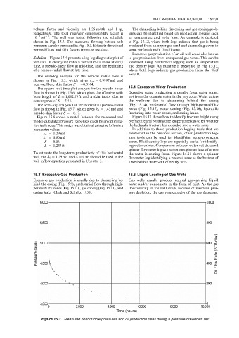
volume factor and viscosity are 1.25 rb/stb and 1 cp, The channeling behind the casing and gas coning prob-
respectively. The total reservoir compressibility factor is lems can be identified based on production logging such
1
10 5 psi . The well was tested following the schedule as temperature and noise logs. An example is depicted
shown in Fig. 15.3. The measured flowing bottom-hole in Fig. 15.12, where both logs indicate that gas is being
pressures are also presented in Fig. 15.3. Estimate directional produced from an upper gas sand and channeling down to
permeabilities and skin factors from the test data. some perforations in the oil zone.
Excessive gas production of an oil well could also be due
Solution Figure 15.4 presents a log-log diagnostic plot of to gas production from unexpected gas zones. This can be
test data. It clearly indicates a vertical radial flow at early identified using production logging such as temperature
time, a pseudo-linear flow at mid-time, and the beginning and density logs. An example is presented in Fig. 15.13,
of a pseudo-radial flow at late time. where both logs indicate gas production from the thief
zone B.
The semi-log analysis for the vertical radial flow is
shown in Fig. 15.5, which gives k yz ¼ 0:9997 md and
near-wellbore skin factor S ¼ 0:0164.
The square-root time plot analysis for the pseudo-linear 15.4 Excessive Water Production
flow is shown in Fig. 15.6, which gives the effective well- Excessive water production is usually from water zones,
bore length of L ¼ 1,082:75 ft and a skin factor due to not from the connate water in the pay zone. Water enters
convergence of S ¼ 3:41. the wellbore due to channeling behind the casing
The semi-log analysis for the horizontal pseudo-radial (Fig. 15.14), preferential flow through high-permeability
flow is shown in Fig. 15.7, which gives k h ¼ 1:43 md and zones (Fig. 15.15), water coning (Fig. 15.16), hydraulic
pseudo-skin factor S ¼ 6:17. fracturing into water zones, and casing leaks.
Figure 15.8 shows a match between the measured and Figure 15.17 shows how to identify fracture height using
model-calculated pressure responses given by an optimiza- prefracture and postfracture temperature logs to tell whether
tiontechnique.This matchwas obtainedusing the following the hydraulic fracture has extended into a water zone.
parameter values: In addition to those production logging tools that are
k h ¼ 1:29 md mentioned in the previous section, other production log-
k z ¼ 0:80 md ging tools can be used for identifying water-producing
S ¼ 0:06 zones. Fluid density logs are especially useful for identify-
L ¼ 1,243 ft: ing water entries. Comparison between water-cut data and
spinner flowmeter log can sometimes give an idea of where
To estimate the long-term productivity of this horizontal the water is coming from. Figure 15.18 shows a spinner
well, the k h ¼ 1:29 md and S ¼ 0:06 should be used in the flowmeter log identifying a watered zone at the bottom of
well inflow equation presented in Chapter 3. a well with a water-cut of nearly 50%.

15.3 Excessive Gas Production 15.5 Liquid Loading of Gas Wells
Excessive gas production is usually due to channeling be- Gas wells usually produce natural gas-carrying liquid
hind the casing (Fig. 15.9), preferential flow through high- water and/or condensate in the form of mist. As the gas
permeability zones (Fig. 15.10), gas coning (Fig. 15.11), and flow velocity in the well drops because of reservoir pres-
casing leaks (Clark and Schultz, 1956). sure depletion, the carrying capacity of the gas decreases.

Figure 15.3 Measured bottom-hole pressures and oil production rates during a pressure drawdown test.