Page 242 - Petroleum Production Engineering, A Computer-Assisted Approach

Guo, Boyun / Computer Assited Petroleum Production Engg 0750682701_chap15 Final Proof page 240 22.12.2006 6:14pm

15/240 PRODUCTION ENHANCEMENT
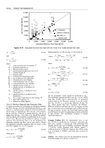
12,000

10,000
Test Flow Rate (Mcf/D) 8,000 Unloaded

6,000

4,000
2,000 ? Nearly loaded up
Loaded up
Questionable
0
0 2,000 4,000 6,000 8,000 10,000 12,000
Calculated Minimum Flow Rate (Mcf/D)
Figure 15.19 Calculated minimum flow rates with the Turner et al. model and test flow rates.

cde
m ¼ , (15:41) Substituting Eq. (15.44) into Eq. (15.34) results in
2
1 þ d e
b
1 2bm m þ n bm 2
and 144ba 1 þ ln a 2 c p ffiffiffi
2 n (15:45)
2
c e
n ¼ , (15:42) tan 1 b 1 tan 1 b 2 ¼ g,
ð 1 þ d eÞ 2
2
where where
A ¼ cross-sectional area of conduit, ft 2 2
D h ¼ hydraulic diameter, in. 5 S g T bh Q gm
a 1 ¼ 9:3 10 p hf , (15:46)
2
f M ¼ Moody friction factor A E km
i
g ¼ gravitational acceleration, 32:17 ft=s 2 2 2
L ¼ conduit length, ft 1:34 10 2 S g T bh Q gm þ m þ n
A 2 E km
p ¼ pressure, psia a 2 ¼ i 2 , (15:47)
p hf ¼ wellhead flowing pressure, psia 144p hf þ m þ n
Q G ¼ gas production rate, Mscf/day 1:34 10 2 S g T bh Q 2 gm þ m
Q o ¼ oil production rate, bbl/day b 1 ¼ p ffiffiffi A 2 E km , (15:48)
i
3
Q s ¼ solid production rate, ft =day n
Q w ¼ water production rate, bbl/day 144p hf þ m
S g ¼ specific gravity of gas, air ¼ 1 b 2 ¼ p ffiffiffi n , (15:49)
S o ¼ specific gravity of produced oil,
freshwater ¼ 1 and
S w ¼ specific gravity of produced water,
2
freshwater ¼ 1 g ¼ a 1 þ d e L: (15:50)
S s ¼ specific gravity of produced solid,
freshwater ¼ 1 All the parameter values should be evaluated at Q gm .
T av ¼ the average temperature in the butting, 8R The minimum required gas flow rate Q gm can be solved
0
« ¼ pipe wall roughness, in. from Eq. (15.45) with a trial-and-error or numerical
u ¼ inclination angle, degrees. method such as the Bisection method. It can be shown
that Eq. (15.45) is a one-to-one function of Q gm for
15.5.2.3 Minimum Required Gas Production Rate Q gm values greater than zero. Therefore, the Newton–
A logical procedure for predicting the minimum required Raphson iteration technique can also be used for solving
gas flow rate Q gm involves calculating gas density r g , gas Q gm . Commercial software packages such as MS Excel can
velocity v g , and gas kinetic energy E k at bottom-hole con- be used as solvers. In fact, the Goal Seek function built
dition using an assumed gas flow rate Q G , and compare into MS Excel was used for generating solutions presented
the E k with E km . If the E k is greater than E km , the Q G is in this chapter. The spreadsheet program is named
higher than the Q gm . The value of Q G should be reduced GasWellLoading.xls.
and the calculation should be repeated until the E k is very
close to E km . Because this procedure is tedious, a simple
equation was derived by Guo et al. for predicting the Example Problem 15.2 To demonstrate how to use
minimum required gas flow rate in this section. Under Eq. (15.45) for predicting the minimum unloading gas
the minimum unloaded condition (the last point of the flow rate, consider a vertical gas well producing 0.70
mist flow regime), Eq. (15.33) becomes specific gravity gas and 50 bbl/day condensate through
a 2.441-in. inside diameter (ID) tubing against a
2
E km ¼ 9:3 10 5 S g T bh Q gm , (15:43) wellhead pressure of 900 psia. Suppose the tubing string
2
A p is set at a depth of 10,000 ft, and other data are given in
i
Table 15.1.
which gives
2
p ¼ 9:3 10 5 S g T bh Q gm : (15:44) Solution The solution given by the spreadsheet program
2
A E km GasWellLoading.xls is shown in Table 15.2.
i