Page 214 - A First Course In Stochastic Models

INSENSITIVITY 207

Denote by j (L) the long-run fraction of type j messages that are lost. Using the
PASTA property, it follows that

c−L−1

1 (L) = p(i 1 , i 2 ) and 2 (L) = p(i 1 , L) + p(i 1 , i 2 )
(i 1 ,i 2 ): i 1 =0 (i 1 ,i 2 ):
i 1 +i 2 =c i 1 +i 2 =c
Since the sum of the average number of messages lost per time unit and the average
number of messages transmitted per time unit equals the arrival rate λ 1 + λ 2 , we
have the identity λ 1 1 (L) + λ 2 2 (L) + T (L) = λ 1 + λ 2 . This relation is useful
as an accuracy check for the calculated values of the p(i 1 , i 2 ). As an illustration,
we consider the following numerical data:

c = 10, λ 1 = 10, λ 2 = 7, µ 1 = 10, µ 2 = 1.
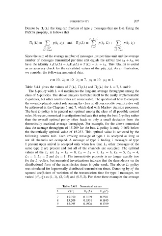
Table 5.4.1 gives the values of T (L), 1 (L) and 2 (L) for L = 7, 8 and 9.
The L-policy with L = 8 maximizes the long-run average throughput among the
class of L-policies. The above analysis restricted itself to the easily implementable
L-policies, but other control rules are conceivable. The question of how to compute
the overall optimal control rule among the class of all conceivable control rules will
be addressed in the Chapters 6 and 7, which deal with Markov decision processes.
The best L-policy is in general not optimal among the class of all possible control
rules. However, numerical investigations indicate that using the best L-policy rather
than the overall optimal policy often leads to only a small deviation from the
theoretically maximal average throughput. For example, for the above numerical
data the average throughput of 15.209 for the best L-policy is only 0.16% below
the theoretically optimal value of 15.233. This optimal value is achieved by the
following control rule. Each arriving message of type 1 is accepted as long as
not all channels are occupied. A message of type 2 finding i messages of type
1 present upon arrival is accepted only when less than L i other messages of the
same type 2 are present and not all of the channels are occupied. The optimal
values of the L i are L 0 = L 1 = 8, L 2 = L 3 = 7, L 4 = 6, L 5 = 5, L 6 = 4,
L 7 = 3, L 8 = 2 and L 9 = 1. The insensitivity property is no longer exactly true
for the L i -policy, but numerical investigations indicate that the dependency on the
distributional form of the transmission times is quite weak. The above L i -policy
2
was simulated for lognormally distributed transmission times. Denoting by c the
i
squared coefficient of variation of the transmission time for type i messages, we
2
2
varied (c , c ) as (1, 1), (2, 0.5) and (0.5, 2). For these three examples the average
1
2
Table 5.4.1 Numerical values
L T (L) 1 (L) 2 (L)
7 15.050 0.0199 0.2501
8 15.209 0.0501 0.1843
9 15.095 0.0926 0.1399