Page 219 - A First Course In Stochastic Models

212 MARKOV CHAINS AND QUEUES

uncompleted service phases present. To find the waiting-time distribution, we need
the customer-average probabilities

π j = the long-run fraction of customers who find j uncompleted
service phases present upon arrival, j = 0, 1, . . . .
Under the assumption of service in order of arrival, let

W q (x) = lim P {D n ≤ x}, x ≥ 0
n→∞
with D n denoting the delay in queue of the nth arriving customer. In the same way
as (5.1.7) was derived in Section 5.1, it can be shown that this limit exists and is
given by
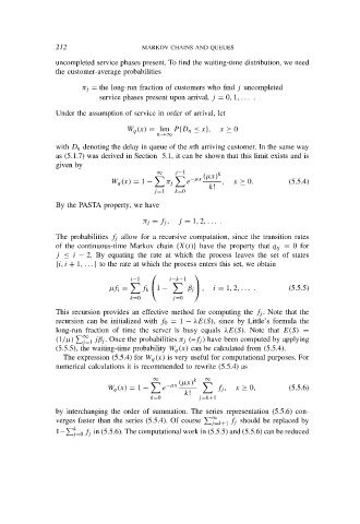
∞ j−1 k
−µx (µx)
W q (x) = 1 − π j e , x ≥ 0. (5.5.4)
k!
j=1 k=0
By the PASTA property, we have

π j = f j , j = 1, 2, . . . .
The probabilities f j allow for a recursive computation, since the transition rates
of the continuous-time Markov chain {X(t)} have the property that q ij = 0 for
j ≤ i − 2. By equating the rate at which the process leaves the set of states
{i, i + 1, . . . } to the rate at which the process enters this set, we obtain
 
i−1 i−k−1

µf i = f k  1 − β j  , i = 1, 2, . . . . (5.5.5)
k=0 j=0
This recursion provides an effective method for computing the f j . Note that the
recursion can be initialized with f 0 = 1 − λE(S), since by Little’s formula the
long-run fraction of time the server is busy equals λE(S). Note that E(S) =
(1/µ) ∞ jβ j . Once the probabilities π j (=f j ) have been computed by applying
j=1
(5.5.5), the waiting-time probability W q (x) can be calculated from (5.5.4).
The expression (5.5.4) for W q (x) is very useful for computational purposes. For
numerical calculations it is recommended to rewrite (5.5.4) as
∞ ∞
−µx (µx) k
W q (x) = 1 − e f j , x ≥ 0, (5.5.6)
k!
k=0 j=k+1
by interchanging the order of summation. The series representation (5.5.6) con-
∞
f
verges faster than the series (5.5.4). Of course j=k+1 j should be replaced by
k
f
1− j=0 j in (5.5.6). The computational work in (5.5.5) and (5.5.6) can be reduced