Page 223 - A First Course In Stochastic Models

216 MARKOV CHAINS AND QUEUES

The routing matrix P = (p ij ), i, j = 1, . . . , K, is assumed to be an irreducible
n
substochastic matrix with the property that P → 0 as n → ∞. Thus each newly
arriving customer ultimately leaves the system with probability 1. To ensure that the
process describing the numbers of customers present at the various stations has an
equilibrium distribution, we need an assumption involving the composite (external
and internal) arrival rates at the stations. Define the composite rates λ 1 , . . . , λ K as
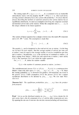
the unique solution to the linear equations

K

λ j = r j + λ i p ij , j = 1, . . . , K. (5.6.1)
i=1
This system of linear equations has a unique solution since the matrix P is transient
and so (I − P) −1 exists. The assumption is made that

λ j
< 1, j = 1, . . . , K. (5.6.2)
µ j
The quantity λ j can be interpreted as the total arrival rate at station j. In the long
run we have for each station i that the average number of arrivals per time unit
at station i must be equal to the average number of service completions per time
unit at station i. In particular, λ i p ij is the arrival rate of customers to station j of
those coming from station i. Hence the total arrival rate at station j must satisfy
(5.6.1). The equations (5.6.1) are called the traffic equations.
For j = 1, . . . , K, define the random variable

X j (t) = the number of customers present at station j at time t.

The multidimensional process X(t) = {(X 1 (t), . . . , X K (t))} is a continuous-time
Markov chain with state space I = {(n 1 , . . . , n K ) | n 1 > 0, . . . , n K > 0}. Since
the routing probability p ii is allowed to be positive, self-transitions can occur in
the process {X(t)}. Under assumption (5.6.2) the process {X(t)} has a unique
equilibrium distribution to be denoted by p(n 1 , . . . , n K ). We now state Theo-
rem 5.6.1.

Theorem 5.6.1 The equilibrium probabilities p(n 1 , . . . , n K ) have the product-
form property

n k
K
λ k λ k

p(n 1 , . . . , n K ) = 1 − . (5.6.3)
µ k µ k
k=1
Proof Let us use the shorthand notation n =(n 1 , . . . , n K ). Let e i denote the ith
unit vector, that is, the ith component of e i is 1 and the other components are zero.
By equating the rate out of state n to the rate into state n (including self-transitions),