Page 221 - A First Course In Stochastic Models

214 MARKOV CHAINS AND QUEUES

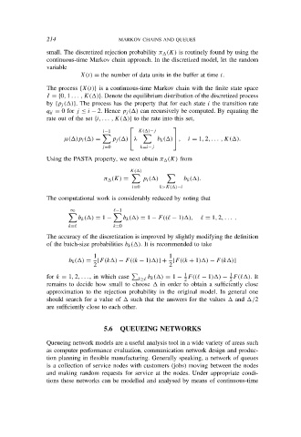
small. The discretized rejection probability π (K) is routinely found by using the
continuous-time Markov chain approach. In the discretized model, let the random
variable
X(t) = the number of data units in the buffer at time t.

The process {X(t)} is a continuous-time Markov chain with the finite state space
I = {0, 1 . . . , K( )}. Denote the equilibrium distribution of the discretized process
by {p j ( )}. The process has the property that for each state i the transition rate
q ij = 0 for j ≤ i − 2. Hence p j ( ) can recursively be computed. By equating the
rate out of the set {i, . . . , K( )} to the rate into this set,
 
i−1 K( )−j

µ( )p i ( ) = p j ( ) λ b k ( ) , i = 1, 2, . . . , K( ).


j=0 k=i−j
Using the PASTA property, we next obtain π (K) from
K( )

π (K) = p i ( ) b k ( ).
i=0 k>K( )−i

The computational work is considerably reduced by noting that
∞ ℓ−1

b k ( ) = 1 − b k ( ) = 1 − F((ℓ − 1) ), ℓ = 1, 2, . . . .
k=ℓ k=0
The accuracy of the discretization is improved by slightly modifying the definition
of the batch-size probabilities b k ( ). It is recommended to take
1 1
b k ( ) = [F(k ) − F((k − 1) )] + [F((k + 1) ) − F(k )]
2 2
1
1
for k = 1, 2, . . . , in which case k≥ℓ k ( ) = 1 − F((ℓ − 1) ) − F(ℓ ). It
b
2
2
remains to decide how small to choose in order to obtain a sufficiently close
approximation to the rejection probability in the original model. In general one
should search for a value of such that the answers for the values and /2
are sufficiently close to each other.
5.6 QUEUEING NETWORKS

Queueing network models are a useful analysis tool in a wide variety of areas such
as computer performance evaluation, communication network design and produc-
tion planning in flexible manufacturing. Generally speaking, a network of queues
is a collection of service nodes with customers (jobs) moving between the nodes
and making random requests for service at the nodes. Under appropriate condi-
tions these networks can be modelled and analysed by means of continuous-time