Page 218 - A First Course In Stochastic Models

A PHASE METHOD 211

of an appropriate continuous-time Markov chain in specific applications. In practice
it is not always obvious how to choose a mixture that is sufficiently close to the
distribution considered. One often confines oneself to a mixture of two Erlangian
distributions by matching only the first two moments of the distribution considered;
see Appendix B.
The phase method is very useful both for theoretical purposes and practical
purposes. We give two examples to illustrate its power.

Example 5.5.1 The M/G/1 queue and the phase method
Customers arrive at a single-server station according to a Poisson process with rate
λ. The service times of the customers are independent and identically distributed
random variables and are also independent of the arrival process. The single server
can handle only one customer at a time and customers are served in order of arrival.
The phase method will be applied to obtain a computationally useful representation
of the waiting-time distribution of a customer when the probability distribution of
the service time of a customer is given by

 
∞ j−1 k
−µx (µx)
P {S ≤ x} = β j  1 − e  , x ≥ 0, (5.5.3)
k!
j=1 k=0
∞
where β j ≥ 0 and j=1 j = 1. The random variable S denotes the service time. It
β
is assumed that λE(S) < 1. In view of (5.5.3) we can think of the service time of a
customer as follows. With probability β j the customer has to go through j sequen-
tial service phases before its service is completed. The phases are processed one
at a time and their durations are independent and exponentially distributed random
variables with mean 1/µ. This interpretation enables us to define a continuous-time
Markov chain. For any t ≥ 0, let

X(t) = the number of uncompleted service phases present at time t.

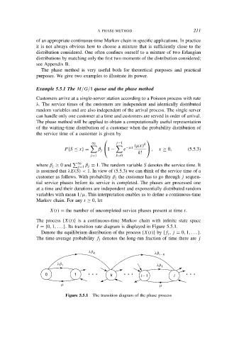
The process {X(t)} is a continuous-time Markov chain with infinite state space
I = {0, 1, . . . }. Its transition rate diagram is displayed in Figure 5.5.1.
Denote the equilibrium distribution of the process {X(t)} by {f j , j = 0, 1, . . . }.
The time-average probability f j denotes the long-run fraction of time there are j

lb k lb i − k

lb 1
lb 1
0 1 • • • k • • • i − 1 i • • •

m m

Figure 5.5.1 The transition diagram of the phase process