Page 87 - A Guide to MATLAB for Beginners and Experienced Users

68 Chapter 5: MATLAB Graphics

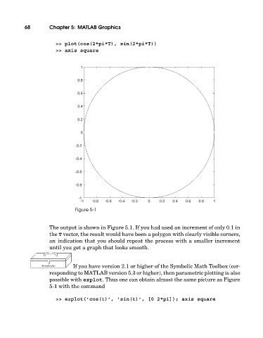
>> plot(cos(2*pi*T), sin(2*pi*T))
>> axis square

1

0.8

0.6

0.4

0.2

0

-0.2

-0.4

-0.6

-0.8

-1
-1 -0.8 -0.6 -0.4 -0.2 0 0.2 0.4 0.6 0.8 1
Figure 5-1

The output is shown in Figure 5.1. If you had used an increment of only 0.1in
the T vector, the result would have been a polygon with clearly visible corners,
an indication that you should repeat the process with a smaller increment
until you get a graph that looks smooth.

If you have version 2.1 or higher of the Symbolic Math Toolbox (cor-
responding to MATLAB version 5.3 or higher), then parametric plotting is also
possible with ezplot. Thus one can obtain almost the same picture as Figure
5-1 withthe command

>> ezplot(’cos(t)’, ’sin(t)’, [0 2*pi]); axis square