Page 23 - A Practical Companion to Reservoir Stimulation

PRACTICAL COMPANION TO RESERVOIR STIMULATION

EXAMPLE A-5
~
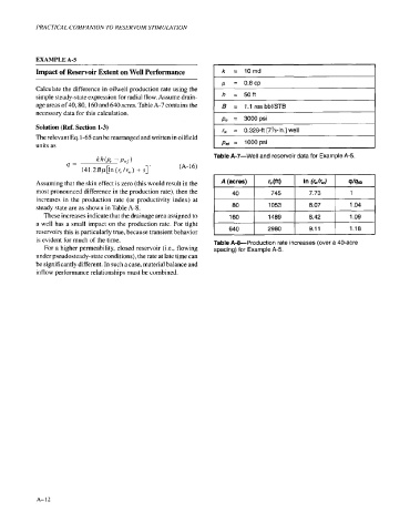
Impact of Reservoir Extent on Well Performance k = 10md
,u = 0.8 cp
Calculate the difference in oilwell production rate using the
simple steady-state expression for radial flow. Assume drain- h = 50ft
age areas of 40,80, 160 and 640 acres. Table A-7 contains the I B = 1.1 res bbl/STB I
necessary data for this calculation.
I pe = 3000 psi I
Solution (Ref. Section 1-3) r, = 0.3284 [77/-in.] well
The relevant Eq. 1-65 can be rearranged and written in oilfield
units as pwr '= 1000 psi
Table'A-7-Well and reservoir data for Example A-5.

Assuming that the skin effect is zero (this would result in the A (acres) re (ft) In (re&) wq40
most pronounced difference in the production rate), then the 40 745 7.73 1
increases in the production rate (or productivity index) at
steady state are as shown in Table A-8. 80 1053 8.07 1.04
These increases indicate that the drainage area assigned to 160 1489 8.42 1.09
a well has a small impact on the production rate. For tight
reservoirs this is particularly true, because transient behavior 640 2980 9.1 1 1.18
is evident for much of the time. Table A-8-Production rate increases (over a 40-acre
For a higher permeability, closed reservoir (i.e., flowing spacing) for Example A-5.
under pseudosteady-state conditions), the rate at late time can
be significantly different. In such a case, material balance and
inflow performance relationships must be combined.

A-12