Page 510 - Acquisition and Processing of Marine Seismic Data

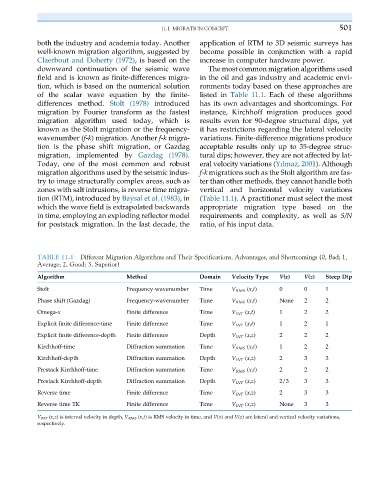
11.1 MIGRATION CONCEPT 501

both the industry and academia today. Another application of RTM to 3D seismic surveys has
well-known migration algorithm, suggested by become possible in conjunction with a rapid
Claerbout and Doherty (1972), is based on the increase in computer hardware power.
downward continuation of the seismic wave The most common migration algorithms used
field and is known as finite-differences migra- in the oil and gas industry and academic envi-
tion, which is based on the numerical solution ronments today based on these approaches are
of the scalar wave equation by the finite- listed in Table 11.1. Each of these algorithms
differences method. Stolt (1978) introduced has its own advantages and shortcomings. For
migration by Fourier transform as the fastest instance, Kirchhoff migration produces good
migration algorithm used today, which is results even for 90-degree structural dips, yet
known as the Stolt migration or the frequency- it has restrictions regarding the lateral velocity
wavenumber (f-k) migration. Another f-k migra- variations. Finite-difference migrations produce
tion is the phase shift migration, or Gazdag acceptable results only up to 35-degree struc-
migration, implemented by Gazdag (1978). tural dips; however, they are not affected by lat-
Today, one of the most common and robust eral velocity variations (Yılmaz, 2001). Although
migration algorithms used by the seismic indus- f-k migrations such as the Stolt algorithm are fas-
try to image structurally complex areas, such as ter than other methods, they cannot handle both
zones with salt intrusions, is reverse time migra- vertical and horizontal velocity variations
tion (RTM), introduced by Baysal et al. (1983),in (Table 11.1). A practitioner must select the most
which the wave field is extrapolated backwards appropriate migration type based on the
in time, employing an exploding reflector model requirements and complexity, as well as S/N
for poststack migration. In the last decade, the ratio, of his input data.

TABLE 11.1 Different Migration Algorithms and Their Specifications, Advantages, and Shortcomings (0, Bad; 1,
Average; 2, Good; 3, Superior)

Algorithm Method Domain Velocity Type V(x) V(z) Steep Dip
Stolt Frequency-wavenumber Time V RMS (x,t) 0 0 1
Phase shift (Gazdag) Frequency-wavenumber Time V RMS (x,t) None 2 2
Omega-x Finite difference Time V INT (x,t) 1 2 2
Explicit finite difference-time Finite difference Time V INT (x,t) 1 2 1
Explicit finite difference-depth Finite difference Depth V INT (x,z) 2 2 2
Kirchhoff-time Diffraction summation Time V RMS (x,t) 1 2 2
Kirchhoff-depth Diffraction summation Depth V INT (x,z) 2 3 3
Prestack Kirchhoff-time Diffraction summation Time V RMS (x,t) 2 2 2
Prestack Kirchhoff-depth Diffraction summation Depth V INT (x,z) 2/3 3 3
Reverse time Finite difference Time V INT (x,z) 2 3 3
Reverse time TK Finite difference Time V INT (x,z) None 3 3
V INT (x,z) is interval velocity in depth, V RMS (x,t) is RMS velocity in time, and V(x) and V(z) are lateral and vertical velocity variations,
respectively.