Page 142 - Adaptive Identification and Control of Uncertain Systems with Nonsmooth Dynamics

138 Adaptive Identification and Control of Uncertain Systems with Non-smooth Dynamics

Remark 9.1. The unknown functions f i (¯x i (t), ¯x i (t − τ ij (t))) in system (9.1)
may not be bounded by the functions of the delayed states. However,
after transforming system (9.1)into(9.4), Assumption 9.1 usually holds
[15,1,2,4]. It should be noted that the bounding functions ϕ ij (·) are not
utilized in the control implementation and thus are not necessarily known.

Remark 9.2. In Assumption 9.2, g i (·) being away from zero is a basic con-
dition for the controlled system (9.4) to avoid the control singularity [1,4].
Without loss of generality, it is assumed that 0 < g i0 ≤ g i (·) ≤ g i1,where the
bounding parameters g i0 and g i1 are only used for analytical purpose.

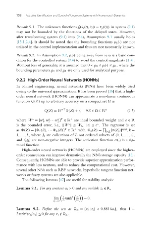
9.2.2 High-Order Neural Networks (HONNs)
In control engineering, neural networks (NNs) have been widely used
owing to the universal approximation. It has been proved [16] that, a high-
order neural network (HONN) can approximate a non-linear continuous
function Q(Z) up to arbitrary accuracy on a compact set as

Q(Z) = W ∗T (Z) + ε, ∀Z ∈ ⊂ R n (9.5)

∗ T
L
where W =[w ,w ···w ] ∈ R are ideal bounded weight and ε ∈ R
∗
∗
∗
1 2 L
is the bounded error, i.e., W ≤ W N , |ε| ≤ ε . The regressor is set
∗
∗
T L d k (j)
as (Z) =[ 1 (Z),··· L (Z)] ∈ R with k (Z) = [σ(Z j )] ,k =
j∈J k
1,...,L,where J k are collections of L not ordered subsets of {0,1,...,n},
and d k (j) are non-negative integers. The activation function σ(·) is a sig-
moid function.
High-order neural networks (HONNs) are employed since the higher-
order connections can improve dramatically the NN’s storage capacity [16].
Consequently, HONNs are able to provide superior approximation perfor-
mance with less neurons, and to reduce the computational cost. However,
several other NNs such as RBF networks, hyperbolic tangent function net-
works or fuzzy systems are also applicable.
The following lemmas [17] are useful for stability analysis:
Lemma 9.1. For any constant ω i > 0 and any variable z i ∈ R,

lim 1 tanh 2 z i = 0.
z i →0 z i ω i
={z i ||z i | < 0.8814ω i },then 1 −
Lemma 9.2. Define the sets as z i
2
2tanh (z i /ω i ) ≤ 0 for any z i /∈ z i .