Page 593 - Advanced_Engineering_Mathematics o'neil

16.2 Wave Motion on an Interval 573

1.5

1

0.5

0
0 0.5 1 1.5 2 2.5 3
x
–0.5

–1
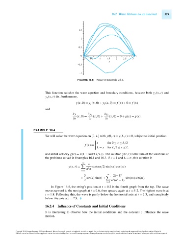
FIGURE 16.5 Waves in Example 16.4.

This function satisfies the wave equation and boundary conditions, because both y f (x,t) and
y g (x,t) do. Furthermore,
y(x,0) = y f (x,0) + y g (x,0) = f (x) + 0 = f (x)
and
∂y ∂y f ∂y g
(x,0) = (x,0) + (x,0) = 0 + g(x) = g(x).
∂t ∂t ∂t

EXAMPLE 16.4
We will solve the wave equation on [0, L] with y(0,t) = y(L,t) = 0, subject to initial position

x for 0 ≤ x ≤ L/2
f (x) =
L − x for L/2 ≤ x ≤ L.
and initial velocity g(x) = x(1 + cos(πx/L)). The solution y(x,t) is the sum of the solutions of
the problems solved in Examples 16.1 and 16.3. If c = 1 and L = π, this solution is

∞

4
y(x,t) = sin(nπ/2)sin(nx)cos(nt)
2
n π
n=1
∞ n
3
2(−1)
+ sin(x)sin(t) + sin(nx)sin(nt).
2
2 n (n − 1)
2
n=2
In Figure 16.5, the string’s position at t = 0.2 is the fourth graph from the top. The wave
moves upward to the next graph at t = 0.6, then upward again at t = 1.2. The highest wave is at
t = 1.8. Following this, the wave is partly below the horizontal axis at t = 2.3, and completely
below this axis at t = 2.9.
16.2.4 Influence of Constants and Initial Conditions
It is interesting to observe how the initial conditions and the constant c influence the wave
motion.

Copyright 2010 Cengage Learning. All Rights Reserved. May not be copied, scanned, or duplicated, in whole or in part. Due to electronic rights, some third party content may be suppressed from the eBook and/or eChapter(s).
Editorial review has deemed that any suppressed content does not materially affect the overall learning experience. Cengage Learning reserves the right to remove additional content at any time if subsequent rights restrictions require it.

October 14, 2010 15:23 THM/NEIL Page-573 27410_16_ch16_p563-610