Page 595 - Advanced_Engineering_Mathematics o'neil

16.2 Wave Motion on an Interval 575

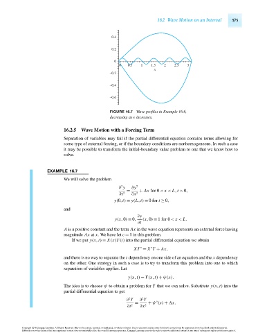
0.4

0.2

0
0 0.5 1 1.5 2 2.5 3
x
–0.2

–0.4

–0.6

FIGURE 16.7 Wave profiles in Example 16.6,
decreasing as increases.

16.2.5 Wave Motion with a Forcing Term
Separation of variables may fail if the partial differential equation contains terms allowing for
some type of external forcing, or if the boundary conditions are nonhomogeneous. In such a case
it may be possible to transform the initial-boundary value problem to one that we know how to
solve.

EXAMPLE 16.7
We will solve the problem
2
∂ y ∂y 2
= + Ax for 0 < x < L,t > 0,
∂t 2 ∂x 2
y(0,t) = y(L,t) = 0for t ≥ 0,
and
∂y
y(x,0) = 0, (x,0) = 1for 0 < x < L.
∂t
A is a positive constant and the term Ax in the wave equation represents an external force having
magnitude Ax at x.Wehavelet c = 1 in this problem.
If we put y(x,t) = X(x)T (t) into the partial differential equation we obtain
XT = X T + Ax,

and there is no way to separate the t dependency on one side of an equation and the x dependency
on the other. One strategy in such a case is to try to transform this problem into one to which
separation of variables applies. Let
y(x,t) = Y(x,t) + ψ(x).
The idea is to choose ψ to obtain a problem for Y that we can solve. Substitute y(x,t) into the
partial differential equation to get
2
2
∂ Y ∂ Y

= + ψ (x) + Ax.
∂t 2 ∂x 2

Copyright 2010 Cengage Learning. All Rights Reserved. May not be copied, scanned, or duplicated, in whole or in part. Due to electronic rights, some third party content may be suppressed from the eBook and/or eChapter(s).
Editorial review has deemed that any suppressed content does not materially affect the overall learning experience. Cengage Learning reserves the right to remove additional content at any time if subsequent rights restrictions require it.

October 14, 2010 15:23 THM/NEIL Page-575 27410_16_ch16_p563-610