Page 767 - Advanced_Engineering_Mathematics o'neil

22.4 Residues and the Inverse Laplace Transform 747

y

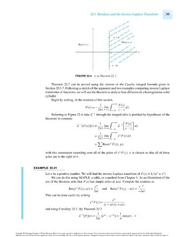
σ + ib
Re(z) > σ
Re(z) < σ

σ x

σ – ib

FIGURE 22.4 σ in Theorem 22.7.

Theorem 22.7 can be proved using the version of the Cauchy integral formula given in
Section 20.3.7. Following a sketch of the argument and two examples computing inverse Laplace
transforms of functions, we will use the theorem to analyze heat diffusion in a homogeneous solid
cylinder.
Begin by writing, in the notation of this section,
1 σ+ib F(z)
F(s) =− lim dz.
2πi b→∞ σ−ib z − s
−1
Referring to Figure 22.4, take L through the integral (this is justified by hypotheses of the
theorem) to compute
1 σ+ib F(z)
−1 −1
L [F(s)](t) = lim L dz
2πi b→∞ σ−ib s − z
1 σ+ib
tz
= lim e F(z)dz
2πi b→∞ σ−ib
tz
= Res(e F(z), p),
p
tz
with this summation extending over all of the poles of e F(z). σ is chosen so that all of these
poles are to the right of σ.

EXAMPLE 22.21
2
2
Let a be a positive number. We will find the inverse Laplace transform of F(z) = 1/(a + z ).
We can do this using MAPLE, a table, or a method from Chapter 3. As an illustration of the
use of the theorem, note that F(z) has simple poles at ±ai. Compute the residues as
e ai e −ai
tz tz
Res(e F(z),ai) = and Res(e F(z),−ai) = .
2ai −2ai
This can be done easily by writing
e tz
tz
e F(z) =
(z − ai)(z + ai)
and using Corollary 22.1. By Theorem 22.7
1
−1 1 ai −ai sin(at).
L [F](t) = e − e =
2ai a

Copyright 2010 Cengage Learning. All Rights Reserved. May not be copied, scanned, or duplicated, in whole or in part. Due to electronic rights, some third party content may be suppressed from the eBook and/or eChapter(s).
Editorial review has deemed that any suppressed content does not materially affect the overall learning experience. Cengage Learning reserves the right to remove additional content at any time if subsequent rights restrictions require it.

October 14, 2010 15:37 THM/NEIL Page-747 27410_22_ch22_p729-750