Page 246 - Advanced Linear Algebra

230 Advanced Linear Algebra

The Operator Adjoint and the Hilbert Space Adjoint
We should make some remarks about the relationship between the operator

adjoint d of , as defined in Chapter 3 and the adjoint i that we have just
defined, which is sometimes called the Hilbert space adjoint . In the first place,
i
if , then ¢= ¦ > d and have different domains and ranges:

d i i and ¢> ¦ = i ¢> ¦ =
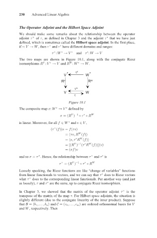
The two maps are shown in Figure 10.1, along with the conjugate Riesz
=
>
i
i
isomorphisms 9¢ = ¦ = and 9 ¢ > ¦ > .
V * W x W *
R V R W
* W
V W
W
Figure 10.1
i
The composite map ¢> ¦ = i defined by
=c k ~²9 ³ i k 9 >
is linear. Moreover, for all  > i and #  = ,

² d ² ³ ³ # ~ ² # ³
>
~º #Á 9 ² ³»

>
~º#Á i 9 ² ³»
=c
i
>
~ ´²9 ³ ² 9 ² ³³µ²#³

~² ³#
i

and so ~ d . Hence, the relationship between d and is

d = c k ~²9 ³ i k 9 >
Loosely speaking, the Riesz functions are like “change of variables” functions
i
from linear functionals to vectors, and we can say that does to Riesz vectors

what d does to the corresponding linear functionals. Put another way (and just
i
as loosely), and are the same, up to conjugate Riesz isomorphism.

In Chapter 3, we showed that the matrix of the operator adjoint d is the
transpose of the matrix of the map . For Hilbert space adjoints, the situation is

slightly different (due to the conjugate linearity of the inner product). Suppose
that 8 and ~² Á Ã Á ³ are ordered orthonormal bases for =
9 ~² Á Ã Á ³

and > , respectively. Then