Page 112 - Advanced engineering mathematics

92 CHAPTER 3 The Laplace Transform

4
2

3 1

–1 0 1 2 3 4 5
2
t
–1
1 –2

–3

0 4 8 12 –4
t
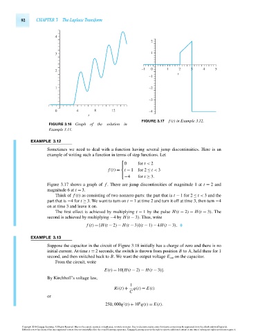
FIGURE 3.17 f (t) in Example 3.12.
FIGURE 3.16 Graph of the solution in
Example 3.11.

EXAMPLE 3.12
Sometimes we need to deal with a function having several jump discontinuities. Here is an
example of writing such a function in terms of step functions. Let
⎧
⎪0 for t < 2
⎨
f (t) = t − 1 for 2 ≤ t < 3
⎪
−4 for t ≥ 3.
⎩
Figure 3.17 shows a graph of f . There are jump discontinuities of magnitude 1 at t = 2 and
magnitude 6 at t = 3.
Think of f (t) as consisting of two nonzero parts: the part that is t − 1for 2 ≤ t < 3 and the
part that is −4for t ≥ 3. We want to turn on t − 1 at time 2 and turn it off at time 3, then turn −4
on at time 3 and leave it on.
The first effect is achieved by multiplying t − 1 by the pulse H(t − 2) − H(t − 3).The
second is achieved by multiplying −4by H(t − 3). Thus, write
f (t) =[H(t − 2) − H(t − 3)](t − 1) − 4H(t − 3).

EXAMPLE 3.13
Suppose the capacitor in the circuit of Figure 3.18 initially has a charge of zero and there is no
initial current. At time t = 2 seconds, the switch is thrown from position B to A, held there for 1
second, and then switched back to B. We want the output voltage E out on the capacitor.
From the circuit, write
E(t) = 10[H(t − 2) − H(t − 3)].
By Kirchhoff’s voltage law,
1
Ri(t) + q(t) = E(t)
C
or
6

250,000q (t) + 10 q(t) = E(t).

Copyright 2010 Cengage Learning. All Rights Reserved. May not be copied, scanned, or duplicated, in whole or in part. Due to electronic rights, some third party content may be suppressed from the eBook and/or eChapter(s).
Editorial review has deemed that any suppressed content does not materially affect the overall learning experience. Cengage Learning reserves the right to remove additional content at any time if subsequent rights restrictions require it.

October 14, 2010 14:14 THM/NEIL Page-92 27410_03_ch03_p77-120