Page 108 - Advanced engineering mathematics

88 CHAPTER 3 The Laplace Transform

1

0.5

0 5 10 15 20
t

–0.5

–1
FIGURE 3.10 H(t − π)cos(t).

1
y

0.5

y = 1
0
0 2 4 6 8
t
t
a b
–0.5

–1
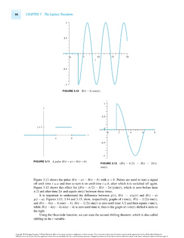
FIGURE 3.11 A pulse H(t − a) − H(t − b).
FIGURE 3.12 (H(t − π/2) − H(t − 2π))
sin(t).

Figure 3.11 shows the pulse H(t − a) − H(t − b) with a < b. Pulses are used to turn a signal
off until time t = a and then to turn it on until time t = b, after which it is switched off again.
Figure 3.12 shows this effect for [H(t − π/2) − H(t − 2π)]sin(t), which is zero before time
π/2 and after time 2π and equals sin(t) between these times.
It is important to understand the difference between g(t), H(t − a)g(t) and H(t − a)
g(t − a). Figures 3.13, 3.14 and 3.15, show, respectively, graphs of t sin(t), H(t − 3/2)t sin(t),
and H(t − 4)(t − 4)sin(t − 4). H(t − 3/2)t sin(t) is zero until time 3/2 and then equals t sin(t),
while H(t − 4)(t − 4)sin(t − 4) is zero until time 4, then is the graph of t sin(t) shifted 4 units to
the right.
Using the Heaviside function, we can state the second shifting theorem, which is also called
shifting in the t variable.

Copyright 2010 Cengage Learning. All Rights Reserved. May not be copied, scanned, or duplicated, in whole or in part. Due to electronic rights, some third party content may be suppressed from the eBook and/or eChapter(s).
Editorial review has deemed that any suppressed content does not materially affect the overall learning experience. Cengage Learning reserves the right to remove additional content at any time if subsequent rights restrictions require it.

October 14, 2010 14:14 THM/NEIL Page-88 27410_03_ch03_p77-120