Page 113 - Advanced engineering mathematics

3.3 Shifting and the Heaviside Function 93

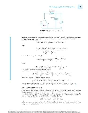
250,000 Ω

1 micro F
A
B E out
10 V

FIGURE 3.18 The circuit of Example
3.13.

We want to solve for q(t) subject to the condition q(0) = 0. Take the Laplace transform of the
differential equation to get
6
250,000[sQ(s) − q(0)]+ 10 Q(s) = L[E(t)].
Now
L[E(t)](s) = 10L[H(t − 2)](s) − 10L[(t − 3)](s)
10 −2s 10 −3s
= e − e .
s s
Now we have an equation for Q:
10 10
5 6 −2s −3s
2.5(10 )sQ(s) + 10 Q(s) = e − e .
s s
Then
1 −2s −5 1 −3s
−5
Q(s) = 4(10 ) e − 4(10 ) e .
s(s + 4) s(s + 4)
Use a partial fractions decomposition to write
1 1 1 1

Q(s) = 10 −5 e −2s − e −2s − 10 −5 e −3s − e −3s .
s s + 4 s s + 4
Applying the second shifting theorem, we get
−5
−5
q(t) = 10 H(t − 2)[1 − e −4(t−2) ]− 10 H(t − 3)[1 − e −4(t−3) ].
Finally, the output voltage is E out (t) = 10 q(t). Figure 3.19 shows a graph of E out (t).
6
3.3.3 Heaviside’s Formula
There is a formula due to Heaviside that can be used to take the inverse transform of a quotient
of polynomials.
Suppose F(s) = p(s)/q(s) with p and q polynomials and q of higher degree than p.We
assume that q can be factored into linear factors and has the form

q(s) = c(s − a 1 )(s − a 2 )···(s − a n ),
with c a nonzero constant and the a j ’s n distinct numbers (which may be real or complex). None
of the a j ’s are roots of p(s).

Copyright 2010 Cengage Learning. All Rights Reserved. May not be copied, scanned, or duplicated, in whole or in part. Due to electronic rights, some third party content may be suppressed from the eBook and/or eChapter(s).
Editorial review has deemed that any suppressed content does not materially affect the overall learning experience. Cengage Learning reserves the right to remove additional content at any time if subsequent rights restrictions require it.

October 14, 2010 14:14 THM/NEIL Page-93 27410_03_ch03_p77-120