Page 88 - Advanced engineering mathematics

68 CHAPTER 2 Linear Second-Order Equations

1

0.5

0
2 4 6 8 10 12 14
t

–0.5

–1
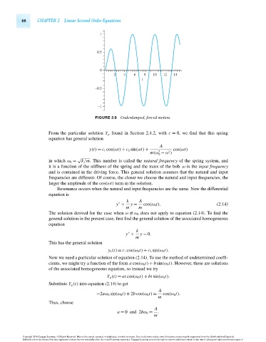
FIGURE 2.9 Underdamped, forced motion.

From the particular solution Y p found in Section 2.4.2, with c = 0, we find that this spring
equation has general solution
A
y(t) = c 1 cos(ωt) + c 2 sin(ωt) + cos(ωt)
2
2
m(ω − ω )
0
√
in which ω 0 = k/m. This number is called the natural frequency of the spring system, and
it is a function of the stiffness of the spring and the mass of the bob. ω is the input frequency
and is contained in the driving force. This general solution assumes that the natural and input
frequencies are different. Of course, the closer we choose the natural and input frequencies, the
larger the amplitude of the cos(ωt) term in the solution.
Resonance occurs when the natural and input frequencies are the same. Now the differential
equation is
k A

y + y = cos(ω 0 t). (2.14)
m m
The solution derived for the case when ω = ω 0 does not apply to equation (2.14). To find the
general solution in the present case, first find the general solution of the associated homogeneous
equation
k

y + y = 0.
m
This has the general solution
y h (t) = c 1 cos(ω 0 t) + c 2 sin(ω 0 t).
Now we need a particular solution of equation (2.14). To use the method of undetermined coeffi-
cients, we might try a function of the form a cos(ω 0 t) + b sin(ω 0 t). However, these are solutions
of the associated homogeneous equation, so instead we try
Y p (t) = at cos(ω 0 t) + bt sin(ω 0 t).
Substitute Y p (t) into equation (2.14) to get
A
−2aω 0 sin(ω 0 t) + 2b cos(ω 0 t) = cos(ω 0 t).
m
Thus, choose
A
a = 0 and 2bω 0 = .
m

Copyright 2010 Cengage Learning. All Rights Reserved. May not be copied, scanned, or duplicated, in whole or in part. Due to electronic rights, some third party content may be suppressed from the eBook and/or eChapter(s).
Editorial review has deemed that any suppressed content does not materially affect the overall learning experience. Cengage Learning reserves the right to remove additional content at any time if subsequent rights restrictions require it.

October 14, 2010 14:12 THM/NEIL Page-68 27410_02_ch02_p43-76