Page 149 - Advances in Biomechanics and Tissue Regeneration

8.3 REDUCED ORDER METHOD 145

i
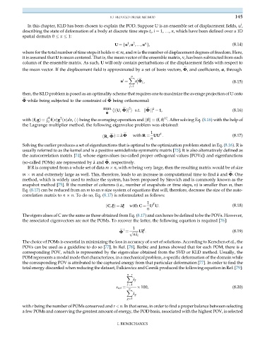
In this chapter, KLD has been chosen to explain the POD. Suppose U is an ensemble set of displacement fields, u ,
describing the state of deformation of a body at discrete time steps t i , i ¼ 1, …, n, which have been defined over a 1D
spatial domain 0 x 1:
n
1
2
U ¼fu ,u ,…,u g, (8.14)
where for the total number of time steps it holds n ≪ m, and m is the number of displacement degrees of freedom. Here,
it is assumed that U is mean centered. That is, the mean vector of the ensemble matrix, v, has been subtracted from each
column of the ensemble matrix. As such, U will only contain perturbations of the displacement fields with respect to

the mean vector. If the displacement field is approximated by a set of basis vectors, Φ, and coefficients, α, through
n
X
i i
j
u ¼ α Φ j , (8.15)
j¼1
then, the KLD problem is posed as an optimality scheme that requires one to maximize the average projection of U onto

Φ while being subjected to the constraint of Φ being orthonormal:

max 2 2 (8.16)
hjðU, ΦÞj i s:t: kΦ k ¼ 1,
Φ
1
R T 12
0
with ðf,gÞ¼ fðxÞg ðxÞdx, h i being the averaging operation and kfk¼ (f, f) . After solving Eq. (8.16) with the help of
the Lagrange multiplier method, the following eigenvalue problem was obtained:
1 T
ðR, Φ Þ¼ λ Φ with R ¼ UU : (8.17)

n
Solving the earlier produces a set of eigenfunctions that is optimal to the optimization problem stated in Eq. (8.16). R is
usually referred to as the kernel and is a positive semidefinite symmetric matrix [73]. It is also alternatively defined as
the autocorrelation matrix [74], whose eigenvalues (so-called proper orthogonal values [POVs]) and eigenfunctions
(so-called POMs) are represented by λ and Φ, respectively.

If R is computed from a whole set of data m n, with m being very large, then the resulting matrix would be of size

m m and extremely large as well. This, therefore, leads to an increase in computational time to find λ and Φ.One
method, which is widely used to reduce the system, has been proposed by Sirovich and is commonly known as the
snapshot method [75]. If the number of columns (i.e., number of snapshots or time steps, n) is smaller than m, then
Eq. (8.17) can be reduced from an m to an n size system of equations that will, therefore, decrease the size of the auto-
correlation matrix to n n. To do so, Eq. (8.17) is reformulated as follows:
1
T
ðC,ξÞ¼ λξ with C ¼ U U: (8.18)
n
The eigenvalues of C are the same as those obtained from Eq. (8.17) and can hence be defined to be the POVs. However,
the associated eigenvectors are not the POMs. To recover the latter, the following equation is required [76]:
1 i
i
Φ ¼ ffiffiffiffiffiffiUξ : (8.19)
p
nλ i
The choice of POMs is essential in minimizing the loss in accuracy of a set of solutions. According to Kerschen et al., the
POVs can be used as a guideline to do so [77]. In Ref. [78], Barbic and James showed that for each POM, there is a
corresponding POV, which is represented by the eigenvalue obtained from the SVD or KLD method. Usually, the
POM represents a modal mode that characterizes, in a mechanical problem, a specific deformation of the domain while
the corresponding POV is attributed to the captured energy from that particular deformation [77]. In order to find the
total energy discarded when reducing the dataset, Falkiewicz and Cesnik produced the following equation in Ref. [79]:

n r
X
λ f
f ¼1
100, (8.20)
ε rel ¼ n
X
λ g
g¼1
with r being the number of POMs conserved and r < n. In that sense, in order to find a proper balance between selecting
a few POMs and conserving the greatest amount of energy, the POD basis, associated with the highest POV, is selected

I. BIOMECHANICS