Page 151 - Advances in Biomechanics and Tissue Regeneration

8.4 WHOLE HEART CYCLE MODELING 147

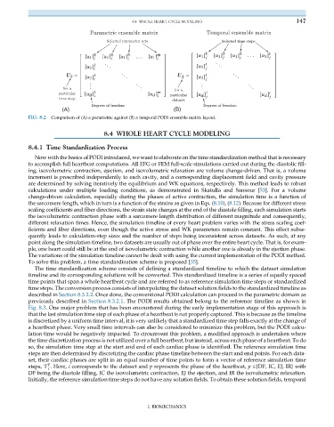
FIG. 8.2 Comparison of (A) a parametric against (B) a temporal PODI ensemble matrix layout.

8.4 WHOLE HEART CYCLE MODELING

8.4.1 Time Standardization Process

Now with the basics of PODI introduced, we want to elaborate on the time standardization method that is necessary
to accomplish full heartbeat computations. All EFG or FEM full-scale simulations carried out during the diastolic fill-
ing, isovolumetric contraction, ejection, and isovolumetric relaxation are volume change-driven. That is, a volume
increment is prescribed independently to each cavity, and a corresponding displacement field and cavity pressure
are determined by solving iteratively the equilibrium and WK equations, respectively. This method leads to robust
calculations under multiple loading conditions, as demonstrated in Skatulla and Sansour [53]. For a volume
change-driven calculation, especially during the phases of active contraction, the simulation time is a function of
the sarcomere length, which in turn is a function of the strains as given in Eqs. (8.10), (8.12). Because for different stress
scaling coefficients and fiber directions, the strain state changes at the end of the diastole filling, each simulation starts
the isovolumetric contraction phase with a sarcomere length distribution of different magnitude and consequently,
different relaxation times. Hence, the simulation timeline of every heart problem varies with the stress scaling coef-
ficients and fiber directions, even though the active stress and WK parameters remain constant. This effect subse-
quently leads to calculation-step sizes and the number of steps being inconsistent across datasets. As such, at any
point along the simulation timeline, two datasets are usually out of phase over the entire heart cycle. That is, for exam-
ple, one heart could still be at the end of isovolumetric contraction while another one is already in the ejection phase.
The variations of the simulation timeline cannot be dealt with using the current implementation of the PODI method.
To solve this problem, a time standardization scheme is proposed [35].
The time standardization scheme consists of defining a standardized timeline to which the dataset simulation
timeline and its corresponding solutions will be converted. This standardized timeline is a series of equally spaced
time points that span a whole heartbeat cycle and are referred to as reference simulation time steps or standardized
time steps. The conversion process consists of interpolating the dataset solution fields to the standardized timeline as
described in Section 8.3.2.2. Once done, the conventional PODI calculation can proceed in the parametric domain as
previously described in Section 8.3.2.1. The PODI results obtained belong to the reference timeline as shown in
Fig. 8.3. One major problem that has been encountered during the early implementation stage of this approach is
that the last simulation time step of each phase of a heartbeat is not properly captured. This is because as the timeline
is discretized by a uniform time interval, it is very unlikely that a standardized time step falls exactly at the change of
a heartbeat phase. Very small time intervals can also be considered to minimize this problem, but the PODI calcu-
lation time would be negatively impacted. To circumvent this problem, a modified approach is undertaken where
the time discretization process is not utilized over a full heartbeat, but instead, across each phase of a heartbeat. To do
so, the simulation time step at the start and end of each cardiac phase is identified. The reference simulation time
steps are then determined by discretizing the cardiac phase timeline between the start and end points. For each data-
set, their cardiac phases are split in an equal number of time points to form a vector of reference simulation time
p
steps, T . Here, i corresponds to the dataset and p represents the phase of the heartbeat, p 2{DF, IC, EJ, IR} with
i
DF being the diastole filling, IC the isovolumetric contraction, EJ the ejection, and IR the isovolumetric relaxation.
Initially, the reference simulation time steps do not have any solution fields. To obtain these solution fields, temporal

I. BIOMECHANICS