Page 156 - Advances in Biomechanics and Tissue Regeneration

152 8. TOWARDS THE REAL-TIME MODELING OF THE HEART

1e+00
1e-03
Magnitude of POV 1e-06

1e-09

1e-12

1e-15
0 1 2 3 4 5 6 7
POV number
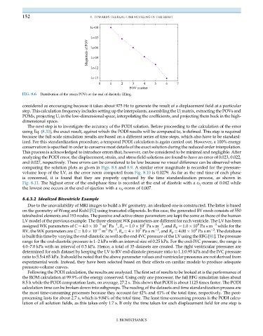
FIG. 8.6 Distribution of the strain POVs at the end of diastolic filling.

considered as encouraging because it takes about 975 Hz to generate the result of a displacement field at a particular
step. This calculation frequency includes setting up the interpolants, assembling the U i matrix, extracting the POVs and
POMs, projecting U i in the low-dimensional space, interpolating the coefficients, and projecting them back in the high-
dimensional space.
The next step is to investigate the accuracy of the PODI solution. Before proceeding to the calculation of the error
using Eq. (8.33), the exact result, against which the PODI results will be compared to, is defined. This step is required
because the full-scale simulation results are based on a different series of time steps, which also have to be standard-
ized. For this standardization procedure, a temporal PODI calculation is again carried out. However, a 100% energy
conservation is specified in order to conserve most details of the exact solution during the reduced order interpolation.
This process is acknowledged to introduce errors that, however, can be considered to be minimal and negligible. After
analyzing the PODI error, the displacement, strain, and stress field solutions are found to have an error of 0.023, 0.022,
and 0.027, respectively. These errors can be considered to be low because no visual difference can be observed when
comparing the solution plots as given in Figs. 8.8 and 8.9. A similar error magnitude is recorded for the pressure-
volume loop of the LV, as the error norm computed from Fig. 8.10 is 0.0279. As far as the end time of each phase
is concerned, it is found that they are properly captured by the time standardization process, as shown in
-norm of 0.042 while
Fig. 8.11. The highest error of the end-phase time is recorded at the end of diastole with a ε ‘ 2
-norm of 0.007.
the lowest one occurs at the end of ejection with a ε ‘ 2
8.4.3.2 Idealized Biventricle Example
Due to the unavailability of MRI images to build a BV geometry, an idealized one is constructed. The latter is based
on the geometry of Wong and Kuhl [52] using truncated ellipsoids. In this case, the generated BV mesh consists of 550
tetrahedral elements and 193 nodes. The passive and active stress parameters are kept the same as those of the human
LV model of the previous example. The three-element WK parameters are different for each ventricle. The LV has been
7
8
1
3
3
assigned WK parameters of C ¼ 4.0 10 9 m Pa , R a ¼ 1.0 10 Pa s m , and R p ¼ 1.0 10 Pa s m 3 while for the
1
3
3
7
3
8
RV, the WK parameters are C ¼ 1.0 10 9 m Pa , R a ¼ 4 10 Pa s m , and R p ¼ 4.00 10 Pa s m . The database
is built this time by varying the end-diastolic as well as the end-IVC pressure of the LV using the EFG [81]. The pressure
range for the end-diastolic pressure is 1–2 kPa with an interval size of 0.25 kPa. For the end-IVC pressure, the range is
4.0–7.0 kPa with an interval of 0.5 kPa. Hence, a total of 35 datasets are created. The right ventricular pressures are
determined for each dataset by keeping the LV to RV end-diastole pressure ratio to 1.1:0.95 kPa and the IVC pressure
ratio to 5.5:4.65 kPa. It should be noted that the above parameter values and ventricular pressures are not derived from
experimental work. Instead, they have been selected based on their effects on cardiac models to produce adequate
pressure-volume curves.
Following the PODI calculation, the results are analyzed. The first set of results to be looked at is the performance of
the ROM calculation at 99.9% of the energy conserved. Using only one processor, the full EFG simulation takes about
8.5 h while the PODI computation lasts, on average, 27.2 s. This shows that PODI is about 1125 times faster. The PODI
calculation time can be broken down into subgroups. The reading of the datasets and time standardization process are
the most time-consuming processes because they account for 42% and 41% of the total time, respectively. The post-
processing lasts for about 2.7 s, which is 9.84% of the total time. The least time-consuming process is the PODI calcu-
lation of all solution fields, as this takes only 1.7 s. If only the time taken for each displacement field for one step is
I. BIOMECHANICS