Page 153 - Advances in Biomechanics and Tissue Regeneration

8.4 WHOLE HEART CYCLE MODELING 149

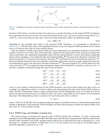
FIG. 8.4 Identification of the phase-change time steps of each phase across a volume-time graph of a dataset, i. Note that the graph is not drawn
to scale.

literature [74]toobtainasmooth transitionof results across aspecific timeframe. In the temporal PODI calculations,
p p
thesupportingtimestepsarefoundin the nonstandardized timeline vector, ½TŠ and are used to interpolate for ½T j Š ,
i i
MLS
where T j is one of the reference time steps. Hence, the MLS interpolants, N time , are defined through:
p
p
½T j Š ¼ N MLS ½TŠ : (8.26)
i time i
Regarding U j , the ensemble data matrix of the temporal PODI calculation, it is constructed as described in
Section 8.3.2.2. With the data matrix and interpolation scheme set up, the temporal PODI calculation can be carried
out for all reference time steps of every selected dataset.
After the datasets’ timeline and solution fields have been standardized, the standardized timeline for the PODI
problem at hand is now created. The current procedure employed is the interpolation of the starting and ending time
steps of each phase, also called phase-change time steps, from the selected datasets. To do so, those phase-change time
SD
SC
steps are first compiled in vectors defined by the start of diastole filling, T ; the start of isovolumetric contraction, T ;
SR
SE
ER
the start of ejection, T ; the start of isovolumetric relaxation, T ; and finally, the end of isovolumetric relaxation, T .
The end of diastole filling, the end of isovolumetric contraction and the end of ejection are not considered because they
SC
SE
are technically the same as the start of isovolumetric contraction, T ; the start of ejection, T ; and the start of isovolu-
SR
metric relaxation, T . For example, the phase-change time steps are first identified for a dataset, i, as shown in Fig. 8.4,
and then compiled in the phase-change time step vectors as follows
SD T SD SD SD
i
m
1
½T Š ¼½T ,…,T ,…,T Š, (8.27)
SC T SC SC SC
m
i
1
½T Š ¼½T ,…,T ,…,T Š, (8.28)
SE T ¼½T ,…,T ,…,T Š, (8.29)
SE
SE
SE
½T Š 1 i m
SR T ¼½T ,…,T ,…,T Š, (8.30)
SR
SR
SR
½T Š 1 i m
ER T ¼½T ,…,T ,…,T Š, (8.31)
ER
ER
ER
½T Š 1 i m
where m is the number of selected datasets for the PODI calculation. Once these phase-change time step vectors are
compiled, an interpolation scheme is carried out along each phase-change time step vector of the PODI problem at
hand. The MLS interpolation scheme is again employed here and the interpolants vector, N, is built up from the
selected dataset parameters because, as indicated earlier, the latter is responsible for the evolution of the simulation
time steps. The interpolation process is carried out for each end-point vector as follows:
^ e e (8.32)
T ¼ N T ,
where e 2{SD, SC, SE, SR, ER}. Once the phase-change time steps of the problem at hand are obtained, the standardized
timeline is determined. The parametric PODI calculation can afterward take place to obtain the solution fields of the
^ e
time steps, T , of the problem at hand.
8.4.2 PODI Usage and Database Construction
This section means to summarize the general usage of PODI coupled with a database. As such, a step-by-step
description of the PODI algorithm is provided. The latter can be split into three main processes: database construction,
reduced order calculation, and finally, postprocessing. Each process is discussed here and accompanied by a work
flowchart of a complete simulation, as illustrated in Fig. 8.5A, and another chart focusing on the detailed steps of
the PODI algorithm, as shown in Fig. 8.5B.
I. BIOMECHANICS