Page 162 - Advances in Biomechanics and Tissue Regeneration

158 8. TOWARDS THE REAL-TIME MODELING OF THE HEART

5
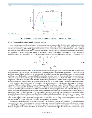
Volume
Number of POMs
80 4

Volume (mL) 60 3 2 Number of POMs conserved

1
40
0
0 0.1 0.2 0.3 0.4 0.5
Time step (s)
FIG. 8.17 Change of the left ventricular volume and number of POMs conserved during one heartbeat.

8.5 PATIENT-SPECIFIC CARDIAC PODI COMPUTATION

8.5.1 Degrees of Freedom Standardization Method

In the previous section, all datasets need to have a common geometry and underlying mesh configuration. In the
case where different geometries and mesh configurations are used, the collated data matrix U i (Eq. 8.21) is ill-set, which
is a crucial shortcoming of the PODI approach. Consider as an example where the PODI calculation is carried out from
five different datasets with geometries of different dimensions as well as meshes and nodal degrees of freedom: model
A ¼ 400 DOFs, model B ¼ 1000 DOFs, model C ¼ 600 DOFs, model D ¼ 2000 DOFs, and model E ¼ 1200 DOFs. Assum-
ing all five models are selected for the PODI computation, then the assembled U i matrix will take the following form:

2 1 2 3 4 5 3
u 1 u 1 u 1 u 1 u 1
⋮ ⋮ ⋮ ⋮ ⋮
6 7
6 1 7
6 u 400 ⋮ ⋮ ⋮ ⋮ 7
⋮ ⋮ ⋮
6 3 7
6 u 7 : (8.34)
U i ¼ 600
6 2 7
u ⋮ ⋮
6 1000 7
⋮
6 5 7
4 u 1200 5
u 4 2000
The type of matrices illustrated in Eq. (8.34) cannot be used for any matrix operations due to incompatible columns due to
the missing matrix entries and the row-wise aligned DOFs not being associated with the same spatial locations. In cardiac
modeling, such problems are likely to be encountered, especially when moving toward the concept of patient-specific
modeling where the heart, for each individual, has distinct anatomical features. Consequently, this research intends to
extend the usage of the PODI technique such that realistic heart geometries can be dealt with. It has to be noted that the
temporal PODI method does not suffer from the incompatible problem as U j is built from a single dataset. That is, the
total number of rows in each column of U j corresponds to the total DOFs of the dataset’s geometry and is thus constant.
In the literature, two recent papers by Amsallem et al. [45] and González et al. [46] have discussed the problem of
extracting POD modes from different mesh configurations. In Amsallem et al., the POMs of different mesh configu-
rations were transformed to the POM, referring to a reference mesh configuration through a minimization process.
However, even though the transformed POMs conserved their orthogonal properties, it is not clear if they also con-
served their optimality properties as being the most dominant modes, and how the whole transformation procedure
impacts the total calculation time. González et al. took a different the approach. The authors embedded different liver
geometries in a benchmark cube mesh grid and computed a so-called distant field with respect to the boundary of the
organ. Following that, a method called locally linear embedding was employed to find the weightage of each regis-
tered liver to reproduce the geometrical shape of the liver at hand and to carry out the interpolation. However, it
remains unclear as to how the nodes inside the liver geometry were treated.
In this research, an alternative approach is proposed that is referred to as the DOFS method. This standardization
procedure, which takes place during the preprocessing stage, consists of projecting the solution fields onto template
nodes [36]. These template nodes are points defined spatially across a template geometry that is the same for every
dataset. The projection itself is based on an interpolation scheme that interpolates the solution fields of the given

I. BIOMECHANICS