Page 163 - Advances in Biomechanics and Tissue Regeneration

8.5 PATIENT-SPECIFIC CARDIAC PODI COMPUTATION 159

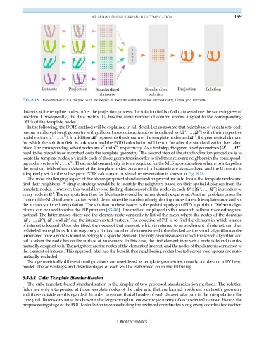
FIG. 8.18 Flowchart of PODI coupled with the degree of freedom standardization method using a cube grid template.

datasets at the template nodes. After the projection process, the solution fields of all datasets share the same degrees of
freedom. Consequently, the data matrix, U i , has the same number of column entries aligned to the corresponding
DOFs of the template nodes.
In the following, the DOFS method will be explained in full detail. Let us assume that a database of N datasets, each
1
N
having a different heart geometry with different mesh discretizations, is defined as {Ω , …, Ω } with their respective
T
U
N
1
nodal vectors {x , …, x }. In addition, Ω represents the domain of the template nodes and Ω , the geometrical domain
for which the solution field is unknown and the PODI calculation will be run for after the standardization has taken
T
1
U
N
place. The corresponding sets of nodes are x and x , respectively. As a first step, the given heart geometries {Ω , …, Ω }
need to be placed in or morphed onto the template geometry. The second step of the standardization procedure is to
T
locate the template nodes, x , inside each of those geometries in order to find their relevant neighbors in the correspond-
1
N
ing nodal vectors {x , …, x }. These nodal connectivity lists are required for the MLS approximation scheme to interpolate
the solution fields of each dataset at the template nodes. As a result, all datasets are standardized and the U i matrix is
adequately set for the subsequent PODI calculation. A visual representation is shown in Fig. 8.18.
The most challenging aspect of the above-proposed standardization procedure is to locate the template nodes and
find their neighbors. A simple strategy would be to identify the neighbors based on their spatial distances from the
N
1
i
template nodes. However, this would involve finding distances of all the nodes in each Ω 2{Ω , …, Ω } in relation to
T
every node in Ω . The computation time for N datasets would be tremendously expensive. Another problem poses the
choice of the MLS influence radius, which determines the number of neighboring nodes for each template node and so,
the accuracy of the interpolation. The solution to these issues is the point-in-polygon (PIP) algorithm. Different algo-
rithms can be used to solve the PIP problem [83–86]. The method employed in this research is the surface orthogonal
method. The latter makes direct use the element-node connectivity list of the mesh where the nodes of the domains
U
1
N
T
{Ω , …, Ω }, Ω ,and Ω are the interconnected vertices. The objective of PIP is to find the element in which a node
of interest is located. Once identified, the nodes of that element, which is referred to as an element of interest, can then
be labeled as neighbors. In this way, only a limited number of elements need to be checked, as the search algorithm can be
terminated once a node is found to belong to a specific element. The only circumstance in which the search algorithm can
fail is when the node lies on the surface of an element. In this case, the first element in which a node is found is auto-
matically assigned to it. The neighbors are the nodes of the element of interest, and the nodes of the elements connected to
the element of interest. This approach also has the benefit that neighboring nodes located across void spaces are auto-
matically excluded.
Two geometrically different configurations are considered as template geometries, namely, a cube and a BV heart
model. The advantages and disadvantages of each will be elaborated on in the following.
8.5.1.1 Cube Template Standardization
The cube template-based standardization is the simpler of two proposed standardization methods. The solution
fields are only interpolated at those template nodes of the cube grid that are located inside each dataset’s geometry
and those outside are disregarded. In order to ensure that all nodes of each dataset take part in the interpolation, the
cube grid dimensions must be chosen to be large enough to encase the geometry of each selected dataset. Hence, the
preprocessing stage of the PODI calculation involves finding the endmost coordinates along every coordinate direction
I. BIOMECHANICS