Page 80 - Advances in Biomechanics and Tissue Regeneration

4.3 MECHANICAL CHARACTERIZATION AND MODELING OF THE AORTA 75

Two ODFs were used to model for the incorporation of anisotropy

• One of the ODFs applied most frequently is 3D bi-π-periodic von Mises ODF for the incorporation of anisotropy in a
microsphere-based model with application to the modeling of the thoracic aorta [7]. This function is expressed as
ρðθÞ¼ ρ ðθÞ + ρ ðθÞ, (4.26)
1
2
where θ ¼ arccosðm rÞ is the so-called mismatch angle and m the preferred mean orientation of the collagen distri-
bution, and
r ffiffiffiffiffi
ρ ðθÞ¼ 4 2π p ffiffiffiffiffi , (4.27)
b expðb½cosð2θÞ +1ŠÞ
i
erfið 2bÞ
where the positive concentration parameter b constitutes a measure of the degree of anisotropy. Moreover, erfi(x) ¼
i erf(x) denotes the imaginary error function. Finally, c 1coll and c 2coll are stress dimensional and dimensionless
material parameters, respectively. A total of five elastic parameters (μ, k 1 , k 2 , κ, and θ) should be fitted.
• We also used the Bingham ODF [41] initially proposed by Alastru e et al. [36] for the incorporation of anisotropy in a
microsphere-based model with application to the modeling of the thoracic aorta and presented in Eq. (4.10).

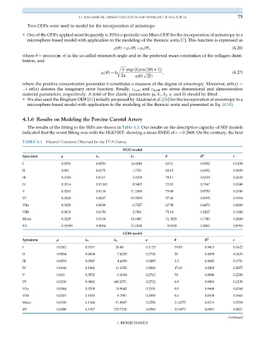
4.3.6 Results on Modeling the Porcine Carotid Artery
The results of the fitting to the SEFs are shown in Table 4.3. Our results on the descriptive capacity of SEF models
indicated that the worst fitting was with the HGO SEF, showing a mean RMSE of ε ¼ 0.2668. On the contrary, the best
TABLE 4.3 Material Constants Obtained for the DTA Curves

HGO model
Specimen μ k 1 k 2 θ R 2 ε
I 0.0531 0.0051 16.4048 63.31 0.9382 0.1458
II 0.001 0.0175 1.7351 80.15 0.6592 0.3459
III 0.0145 0.0117 3.0238 78.11 0.8329 0.2626
IV 0.0314 0.01363 8.5495 72.82 0.7947 0.3048
V 0.0263 0.0134 11.2069 79.88 0.8750 0.2486
VI 0.0435 0.0037 93.9559 57.43 0.8295 0.2316
VIIa 0.0129 0.0038 6.7227 67.58 0.6670 0.4269
VIIb 0.0010 0.0150 2.7861 79.14 0.2827 0.1686
Mean 0.0229 0.0104 18.0481 72.3025 0.7349 0.2668
SD 0.01908 0.0054 31.0638 8.6528 0.2063 0.0919
GOH model
Specimen μ k 1 k 2 κ θ R 2 ε
I 0.0262 0.0117 26.06 0.1125 59.83 0.9415 0.1422
II 0.0054 0.0654 7.6320 0.2726 20 0.6858 0.3431
III 0.0078 0.0947 4.6290 0.2885 1.5 0.8680 0.1701
IV 0.0146 0.1906 11.1502 0.2848 17.69 0.8200 0.2875
V 0.001 0.3552 0.0014 0.2742 74 0.8840 0.2256
VI 0.0210 0.0862 660.0371 0.2712 0.0 0.8494 0.2139
VIIa 0.0064 0.0258 18.9642 0.2531 0.0 0.6668 0.4268
VIIb 0.0025 0.1035 6.7001 0.2895 0.0 0.8558 0.2663
Mean 0.0106 0.1166 91.8967 0.2558 21.6275 0.8214 0.2594
SD 0.0090 0.1107 229.7130 0.0590 29.3472 0.0961 0.0931
Continued
I. BIOMECHANICS