Page 322 -

296 Chapter 8 ■ Classification

values, or a small standard deviation, is desired because it corresponds to an
easier thresholding problem. It would also mean that the feature values would
be less likely to overlap with those of other objects. A large distance between
means of classes to be separated is important, too.
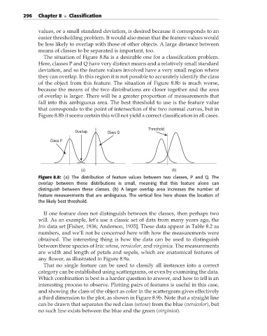
The situation of Figure 8.8a is a desirable one for a classification problem.
Here, classes P and Q have very distinct means and a relatively small standard
deviation, and so the feature values involved have a very small region where
they can overlap. In this region it is not possible to accurately identify the class
of the object from this feature. The situation of Figure 8.8b is much worse,
because the means of the two distributions are closer together and the area
of overlap is larger. There will be a greater proportion of measurements that
fall into this ambiguous area. The best threshold to use is the feature value
that corresponds to the point of intersection of the two normal curves, but in
Figure 8.8b it seems certain this will not yield a correct classification in all cases.

Threshold
Overlap Class Q
Class P

(a) (b)
Figure 8.8: (a) The distribution of feature values between two classes, P and Q. The
overlap between these distributions is small, meaning that this feature alone can
distinguish between these classes. (b) A larger overlap area increases the number of
feature measurements that are ambiguous. The vertical line here shows the location of
the likely best threshold.

If one feature does not distinguish between the classes, then perhaps two
will. As an example, let’s use a classic set of data from many years ago, the
Iris data set [Fisher, 1936; Anderson, 1935]. These data appear in Table 8.2 as
numbers, and we’ll not be concerned here with how the measurements were
obtained. The interesting thing is how the data can be used to distinguish
between three species of Iris: setosa, versicolor,and virginica. The measurements
are width and length of petals and sepals, which are anatomical features of
any flower, as illustrated in Figure 8.9a.
That no single feature can be used to classify all instances into a correct
category can be established using scattergrams, or even by examining the data.
Which combination is best is a harder question to answer, and how to tell is an
interesting process to observe. Plotting pairs of features is useful in this case,
and showing the class of the object as color in the scattergram gives effectively
a third dimension to the plot, as shown in Figure 8.9b. Note that a straight line
can be drawn that separates the red class (setosa)from the blue (versicolor), but
no such line exists between the blue and the green (virginica).