Page 325 -

Chapter 8 ■ Classification 299

(a) (b)
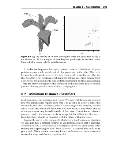
Figure 8.9: (a) The anatomy of a flower, showing the petals and sepals that are key to
the Iris data set. (b) A scattergram of Sepal length vs. petal length for the three classes.
Color codes the classes; note the spatial groupings.

A line breaks the green-blue region into two parts such that almost all green
points are on one side and almost all blue points are on the other. This could
be used to distinguish between the two classes with a small error. The line
that does this is not horizontal, but that does not matter. This is called a linear
discriminant and is commonly used in data classification and machine learning.
There are many references to this technique in the literature. It is, of course,
just one of many possible methods for classifying data.

8.2 Minimum Distance Classifiers

Looking again at the scattergram of Figure 8.9b, note that the data are grouped
into two-dimensional regions such that it is possible to draw a curve that
surrounds each class. Of course, such a curve can get very complex, and the
curve would only surround the points we knew about. A new object and set
of measurements may lie well outside of the curve. If an unknown object is
measured and if the measurements form a point that falls inside that curve,
then it probably should be classified with the others within the curve.
Because the curve is too complex to identify and hard to use as a classifier,
we can introduce a simpler scheme: an unidentified region that is classified
according to how far away it is (as a point) from any of the other points in the
training set. Depending on how ‘‘how far away’’ is defined, this could work
pretty well. This is what is commonly known as distance, and there are several
reasonable ways to define and implement it.