Page 236 -

216 CHAPTER 5 LINEAR PROGRAMMING: THE SIMPLEX METHOD

Can you find basic and foundatanextremepoint.Becauseevery extreme point corresponds to a basic feasible
basic feasible solutions solution, we can now conclude that the HighTech problem does have an optimal basic
to a system of equations 2
at this point? Try feasible solution. The Simplex method is an iterative procedure for moving from one
Problem 1. basic feasible solution (extreme point) to another until the optimal solution is reached.

5.2 Tableau Form

In geometry, a simplex is With the Simplex method, an LP problem and its iterative solutions are usually
an n dimensional presented in tables, or tableau formats. Each tableau represents a basic solution
equivalent of a two from the Simplex procedure. The tableau also provides a convenient method of
dimensional triangle, so
the Simplex method is identifying whether a potentially improved solution exists. If we take our standard
really looking for the LP format from the HighTech problem we have:
corner points in n
dimensions. Max: 50x 1 þ 40x 2 þ 0s 1 þ 0s 2 þ 0s 3
s:t:
¼ 150
3x 1 þ 5x 2 þ 1s 1
1x 2 þ 1s 2 ¼ 20
þ 1s 3 ¼ 300
8x 1 þ 5x 2
x 1 ; x 2 ; s 1 ; s 2 ; s 3 0
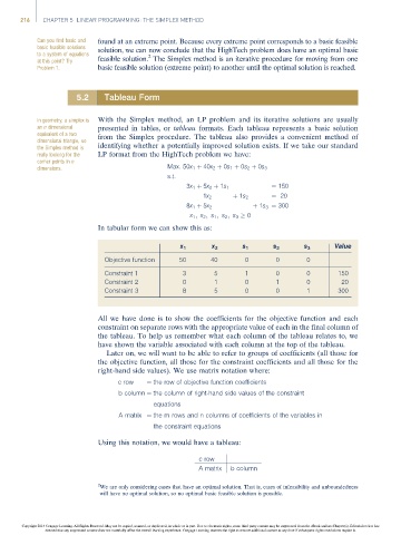
In tabular form we can show this as:

Value
x 1 x 2 s 1 s 2 s 3
Objective function 50 40 0 0 0
Constraint 1 3 5 1 0 0 150
Constraint 2 0 1 0 1 0 20
Constraint 3 8 5 0 0 1 300

All we have done is to show the coefficients for the objective function and each
constraint on separate rows with the appropriate value of each in the final column of
the tableau. To help us remember what each column of the tableau relates to, we
have shown the variable associated with each column at the top of the tableau.
Later on, we will want to be able to refer to groups of coefficients (all those for
the objective function, all those for the constraint coefficients and all those for the
right-hand side values). We use matrix notation where:
c row ¼ the row of objective function coefficients
b column ¼ the column of right-hand side values of the constraint
equations
A matrix ¼ the m rows and n columns of coefficients of the variables in
the constraint equations

Using this notation, we would have a tableau:

c row
A matrix b column

2
We are only considering cases that have an optimal solution. That is, cases of infeasibility and unboundedness
will have no optimal solution, so no optimal basic feasible solution is possible.

Copyright 2014 Cengage Learning. All Rights Reserved. May not be copied, scanned, or duplicated, in whole or in part. Due to electronic rights, some third party content may be suppressed from the eBook and/or eChapter(s). Editorial review has
deemed that any suppressed content does not materially affect the overall learning experience. Cengage Learning reserves the right to remove additional content at any time if subsequent rights restrictions require it.