Page 240 -

220 CHAPTER 5 LINEAR PROGRAMMING: THE SIMPLEX METHOD

profitability). So, to calculate the change in the objective function, if we increase x 1
by 1 we would have:
z 1 ¼ 0ð3Þþ 0ð0Þþ 0ð8Þ¼ 0
Here we multiply the objective function coefficient of the relevant basic variable by
the change in the value of that variable. This increases x 1 by 1. Clearly the net effect
on the objective function is zero – reducing the value of s 1 , s 2 and s 3 will have a zero
effect on the objective function value. The comparable calculations for the other z j
values are then:
z 2 ¼ 0ð5Þþ 0ð1Þþ 0ð5Þ¼ 0
z 3 ¼ 0ð1Þþ 0ð0Þþ 0ð0Þ¼ 0
z 4 ¼ 0ð0Þþ 0ð1Þþ 0ð0Þ¼ 0
z 5 ¼ 0ð0Þþ 0ð0Þþ 0ð1Þ¼ 0

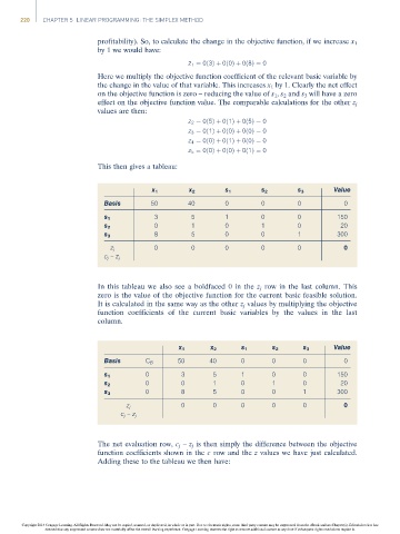
This then gives a tableau:

Value
x 1 x 2 s 1 s 2 s 3
Basis 50 40 0 0 0 0
3 5 1 0 0 150
s 1
0 1 0 1 0 20
s 2
8 5 0 0 1 300
s 3
0 0 0 0 0 0
z j
c j –z j

In this tableau we also see a boldfaced 0 in the z j row in the last column. This
zero is the value of the objective function for the current basic feasible solution.
It is calculated in the same way as the other z j values by multiplying the objective
function coefficients of the current basic variables by the values in the last
column.

Value
x 1 x 2 s 1 s 2 s 3
Basis C B 50 40 0 0 0 0

s 1 0 3 5 1 0 0 150
s 2 0 0 1 0 1 0 20
s 3 0 8 5 0 0 1 300
0 0 0 0 0 0
z j
c j –z j

The net evaluation row, c j – z j is then simply the difference between the objective
function coefficients shown in the c row and the z values we have just calculated.
Adding these to the tableau we then have:

Copyright 2014 Cengage Learning. All Rights Reserved. May not be copied, scanned, or duplicated, in whole or in part. Due to electronic rights, some third party content may be suppressed from the eBook and/or eChapter(s). Editorial review has
deemed that any suppressed content does not materially affect the overall learning experience. Cengage Learning reserves the right to remove additional content at any time if subsequent rights restrictions require it.