Page 245 -

CALCULATING THE NEXT TABLEAU 225

with a corresponding profit of E0. One iteration of the Simplex method moved us to
another basic feasible solution with an objective function value of E1875. This new
basic feasible solution is:
x 1 ¼ 37:5
x 2 ¼ 0
s 1 ¼ 37:5
s 2 ¼ 20
s 3 ¼ 0
In Figure 5.2 we see that the initial basic feasible solution corresponds to extreme
point*1 . The first iteration moved us in the direction of the greatest increase per
unit in profit – that is, along the x 1 axis. We moved away from extreme point*1in
The first iteration moves the x 1 direction until we could move no farther without violating one of the con-
us from the origin in
Figure 5.2 to extreme straints. The tableau we obtained after one iteration provides the basic feasible
point 2. solution corresponding to extreme point*2.
We note from Figure 5.2 that at extreme point *2 the warehouse capacity
constraint is binding with s 3 ¼ 0 and that the other two constraints contain slack.
From the simplex tableau, we see that the amount of slack for these two constraints
is given by s 1 ¼ 37.5 and s 2 ¼ 20.

Moving Toward a Better Solution
To see whether a better basic feasible solution can be found, we need again to
calculate the z j and c j – z j rows for the new simplex tableau. Recall that the elements
in the z j row are the sum of the products obtained by multiplying the elements in the
c B column of the simplex tableau by the corresponding elements in the columns of
the A matrix. Thus, we obtain:

z 1 ¼ 0ð0Þ þ 0ð0Þþ 50ð1Þ ¼ 50
z 2 ¼ 0ð31:25Þþ 0ð1Þþ 50ð0:625Þ¼ 31:25
z 3 ¼ 0ð1Þ þ 0ð0Þþ 50ð0Þ ¼ 0
z 4 ¼ 0ð0Þ þ 0ð1Þþ 50ð0Þ ¼ 0
z 5 ¼ð 0:375Þþ 0ð0Þþ 50ð0:125Þ¼ 6:25

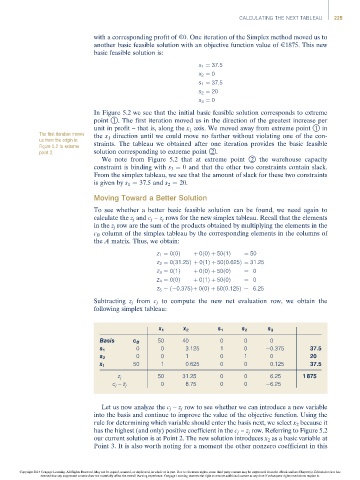
Subtracting z j from c j to compute the new net evaluation row, we obtain the
following simplex tableau:

x 1 x 2 s 1 s 2 s 3
Basis c B 50 40 0 0 0
0 0 3.125 1 0 0.375 37.5
s 1
0 0 1 0 1 0 20
s 2
50 1 0.625 0 0 0.125 37.5
x 1
z j 50 31.25 0 0 6.25 1 875
c j – z j 0 8.75 0 0 6.25

Let us now analyze the c j – z j row to see whether we can introduce a new variable
into the basis and continue to improve the value of the objective function. Using the
rule for determining which variable should enter the basis next, we select x 2 because it
has the highest (and only) positive coefficient in the c j – z j row. Referring to Figure 5.2
our current solution is at Point 2. The new solution introduces x 2 as a basic variable at
Point 3. It is also worth noting for a moment the other nonzero coefficient in this

Copyright 2014 Cengage Learning. All Rights Reserved. May not be copied, scanned, or duplicated, in whole or in part. Due to electronic rights, some third party content may be suppressed from the eBook and/or eChapter(s). Editorial review has
deemed that any suppressed content does not materially affect the overall learning experience. Cengage Learning reserves the right to remove additional content at any time if subsequent rights restrictions require it.