Page 243 -

CALCULATING THE NEXT TABLEAU 223

We know that x 1 is set to enter the new solution and that s 3 is set to leave. We refer
to the x 1 column as the pivot column, the s 3 row as the pivot row and the coefficient
at the intersection of the pivot row and column as the pivot element (here 8, shown
circled). Looking at the pivot row we have:

8x 1 þ 5x 2 þ 1s 3 ¼ 300

We know that in the improved solution, x 1 will enter the solution and that both x 2
and s 3 will be non-basic and take zero values. Given that, in the above equation we
know that two of the variables will be zero, we can easily solve for the third, x 1 ,by
dividing the entire row by 8, the pivot element:
8x 1 5x 2 1s 3 300
þ þ ¼
8 8 8 8
This gives:

1x 1 þ 0:625x 2 þ 0:125s 3 ¼ 37:5
This row replaces the existing pivot row in the new tableau.

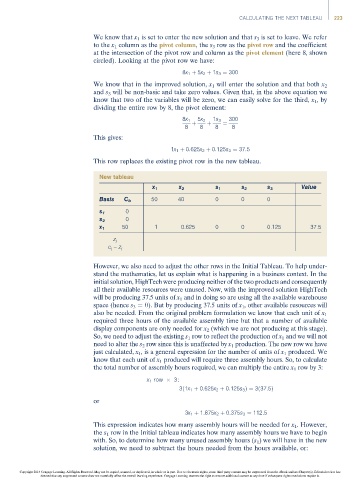
New tableau
Value
x 1 x 2 s 1 s 2 s 3
Basis C b 50 40 0 0 0

s 1 0
s 2 0
x 1 50 1 0.625 0 0 0.125 37.5
z j
c j –z j

However, we also need to adjust the other rows in the Initial Tableau. To help under-
stand the mathematics, let us explain what is happening in a business context. In the
initial solution, HighTech were producing neither of the two products and consequently
all their available resources were unused. Now, with the improved solution HighTech
will be producing 37.5 units of x 1 and in doing so are using all the available warehouse
space (hence s 3 ¼ 0). But by producing 37.5 units of x 1 , other available resources will
also be needed. From the original problem formulation we know that each unit of x 1
required three hours of the available assembly time but that a number of available
display components are only needed for x 2 (which we are not producing at this stage).
So, we need to adjust the existing s 1 row to reflect the production of x 1 and we will not
need to alter the s 2 row since this is unaffected by x 1 production. The new row we have
just calculated, x 1 , is a general expression for the number of units of x 1 produced. We
know that each unit of x 1 produced will require three assembly hours. So, to calculate
the total number of assembly hours required, we can multiply the entire x 1 row by 3:

x 1 row 3:
3ð1x 1 þ 0:625x 2 þ 0:125s 3 Þ¼ 3ð37:5Þ

or
3x 1 þ 1:875x 2 þ 0:375s 3 ¼ 112:5
This expression indicates how many assembly hours will be needed for x 1 . However,
the s 1 row in the Initial tableau indicates how many assembly hours we have to begin
with. So, to determine how many unused assembly hours (s 1 ) we will have in the new
solution, we need to subtract the hours needed from the hours available, or:

Copyright 2014 Cengage Learning. All Rights Reserved. May not be copied, scanned, or duplicated, in whole or in part. Due to electronic rights, some third party content may be suppressed from the eBook and/or eChapter(s). Editorial review has
deemed that any suppressed content does not materially affect the overall learning experience. Cengage Learning reserves the right to remove additional content at any time if subsequent rights restrictions require it.