Page 244 -

224 CHAPTER 5 LINEAR PROGRAMMING: THE SIMPLEX METHOD

Assembly hours available 3x 1 + 5x 2 +1s 1 +0s 2 + 0s 3 ¼ 150
– assembly hours needed for x 1 –(3x 1 + 1.875x 2 + .375s 3 ¼ 112.5)
production
0x 1 + 3.125x 2 +1s 1 +0s 2 – 0.375s 3 ¼ 37.5
Giving s 1

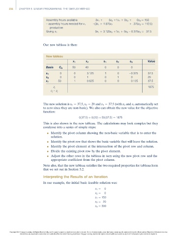
Our new tableau is then:

New tableau
x 1 x 2 s 1 s 2 s 3 Value
Basis C b 50 40 0 0 0

0 0 3.125 1 0 0.375 37.5
s 1
0 0 1 0 1 0 20
s 2
x 1 50 1 0.625 0 0 0.125 37.5
z j 1875
c j –z j

The new solution is s 1 ¼ 37.5, s 2 ¼ 20 and x 1 ¼ 37.5 (with x 2 and s 3 automatically set
to zero since they are non-basic). We also can obtain the new value for the objective
function:

0ð37:5Þþ 0ð20Þþ 50ð37:5Þ¼ 1875
This is also shown in the new tableau. The calculations may look complex but they
condense into a series of simple steps:

l Identify the pivot column showing the non-basic variable that is to enter the
solution.
l Identify the pivot row that shows the basic variable that will leave the solution.
l Identify the pivot element at the intersection of the pivot row and column.
l Divide the existing pivot row by the pivot element.
l Adjust the other rows in the tableau in turn using the new pivot row and the
appropriate coefficient from the pivot column.
Note also, that the new tableau satisfies the two required properties for tableau form
that we set out in Section 5.2.

Interpreting the Results of an Iteration
In our example, the initial basic feasible solution was:
x 1 ¼ 0
x 2 ¼ 0
s 1 ¼ 150
s 2 ¼ 20
s 3 ¼ 300

Copyright 2014 Cengage Learning. All Rights Reserved. May not be copied, scanned, or duplicated, in whole or in part. Due to electronic rights, some third party content may be suppressed from the eBook and/or eChapter(s). Editorial review has
deemed that any suppressed content does not materially affect the overall learning experience. Cengage Learning reserves the right to remove additional content at any time if subsequent rights restrictions require it.