Page 247 -

CALCULATING THE NEXT TABLEAU 227

With 12 as the minimum ratio, s 1 will leave the basis. The pivot element is
a 12 ¼ 3.125, which is circled in the preceding tableau. The nonbasic variable x 2 must
now be made a basic variable.
We can make this change by performing the following elementary row
operations:
Step 1. Divide every element in row 1 (the pivot row) by 3.125 (the pivot
element).
Step 2. Subtract the new row 1 (the new pivot row) from row 2.
Step 3. Multiply the new pivot row by 0.625, and subtract the result from
row 3.
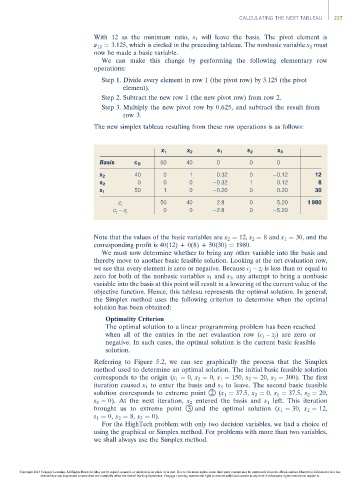
The new simplex tableau resulting from these row operations is as follows:

x 1 x 2 s 1 s 2 s 3
Basis c B 50 40 0 0 0
40 0 1 0.32 0 0.12 12
x 2
0 0 0 0.32 1 0.12 8
s 2
50 1 0 0.20 0 0.20 30
x 1
z j 50 40 2.8 0 5.20 1 980
c j – z j 0 0 2.8 0 5.20

Note that the values of the basic variables are x 2 ¼ 12, s 2 ¼ 8 and x 1 ¼ 30, and the
corresponding profit is 40(12) + 0(8) + 50(30) ¼ 1980.
We must now determine whether to bring any other variable into the basis and
thereby move to another basic feasible solution. Looking at the net evaluation row,
we see that every element is zero or negative. Because c j – z j is less than or equal to
zero for both of the nonbasic variables s 1 and s 3 , any attempt to bring a nonbasic
variable into the basis at this point will result in a lowering of the current value of the
objective function. Hence, this tableau represents the optimal solution. In general,
the Simplex method uses the following criterion to determine when the optimal
solution has been obtained:
Optimality Criterion
The optimal solution to a linear programming problem has been reached
when all of the entries in the net evaluation row (c j – z j ) are zero or
negative. In such cases, the optimal solution is the current basic feasible
solution.
Referring to Figure 5.2, we can see graphically the process that the Simplex
method used to determine an optimal solution. The initial basic feasible solution
corresponds to the origin (x 1 ¼ 0, x 2 ¼ 0, s 1 ¼ 150, s 2 ¼ 20, s 3 ¼ 300). The first
iteration caused x 1 to enterthe basisand s 3 to leave. The second basic feasible
solution corresponds to extreme point *2(x 1 ¼ 37.5, x 2 ¼ 0, s 1 ¼ 37.5, s 2 ¼ 20,
s 3 ¼ 0). At the next iteration, x 2 entered the basis and s 1 left. This iteration
brought us to extreme point *3 and the optimal solution (x 1 ¼ 30, x 2 ¼ 12,
s 1 ¼ 0, s 2 ¼ 8, s 3 ¼ 0).
For the HighTech problem with only two decision variables, we had a choice of
using the graphical or Simplex method. For problems with more than two variables,
we shall always use the Simplex method.

Copyright 2014 Cengage Learning. All Rights Reserved. May not be copied, scanned, or duplicated, in whole or in part. Due to electronic rights, some third party content may be suppressed from the eBook and/or eChapter(s). Editorial review has
deemed that any suppressed content does not materially affect the overall learning experience. Cengage Learning reserves the right to remove additional content at any time if subsequent rights restrictions require it.