Page 34 -

14 CHAPTER 1 INTRODUCTION

In general, experimenting with models requires less time and is less expensive than
experimenting with the real object or situation. A model aeroplane is certainly quicker
and less expensive to build and study than the full-size aeroplane. Similarly, the
mathematical model in Equation (1.1) allows a quick identification of profit expect-
ations without actually requiring the manager to produce and sell 300 units. Models
also have the advantage of reducing the risk associated with experimenting with the
real situation. In particular, bad designs or bad decisions that cause the model aero-
plane to crash or a mathematical model to project a E10000 loss can be avoided in the
real situation. The value of model-based conclusions and decisions is dependent on
how well the model represents the real situation. The more closely the model
aeroplane represents the real aeroplane the more accurate the conclusions and
predictions will be. Similarly, the more closely the mathematical model represents
the company’s true profit-volume relationship, the more accurate the profit pro-
jections will be.
Obviously our model in equation (1.1) is quite simple and basic – it consists of
only one equation after all. To illustrate some additional aspects of MS models
we’ll expand the situation. Let us assume that management have agreed, during
the problem structuring and definition phase, that their problem is to maximize
the company’s profit, P. However, they have also identified certain factors that
must be taken into account when seeking to maximize profit. One critical
requirement relates to the fact that each unit of the item produced by the
company takes five hours of production time and that each day there are only
40 hoursof production time available given theexistingworkforce.Wecan show
the company’s objective mathematically as:

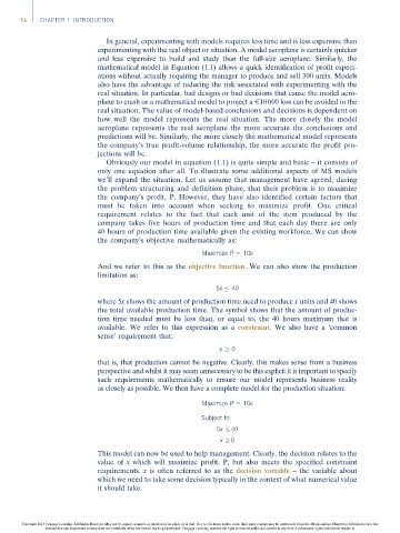
Maximize P =10x
And we refer to this as the objective function. We can also show the production
limitation as:

5x 40
where 5x shows the amount of production time need to produce x units and 40 shows
the total available production time. The symbol shows that the amount of produc-
tion time needed must be less than, or equal to, the 40 hours maximum that is
available. We refer to this expression as a constraint. We also have a ‘common
sense’ requirement that:
x 0

that is, that production cannot be negative. Clearly, this makes sense from a business
perspective and whilst it may seem unnecessary to be this explicit it is important to specify
such requirements mathematically to ensure our model represents business reality
as closely as possible. We then have a complete model for the production situation:

Maximize P =10x
Subject to:
5x 40
x 0
This model can now be used to help management. Clearly, the decision relates to the
value of x which will maximize profit, P, but also meets the specified constraint
requirements. x is often referred to as the decision variable – the variable about
which we need to take some decision typically in the context of what numerical value
it should take.

Copyright 2014 Cengage Learning. All Rights Reserved. May not be copied, scanned, or duplicated, in whole or in part. Due to electronic rights, some third party content may be suppressed from the eBook and/or eChapter(s). Editorial review has
deemed that any suppressed content does not materially affect the overall learning experience. Cengage Learning reserves the right to remove additional content at any time if subsequent rights restrictions require it.