Page 442 -

422 CHAPTER 10 INVENTORY MODELS

the inventory model with backorders, we encounter the usual holding costs and
ordering costs. We also incur a backorder cost in terms of the labour and
special delivery costs directly associated with the handling of the backorders.
Another element of the backorder cost accounts for the loss of goodwill
because some customers will have to wait for their orders. Because the good-
will cost depends on how long a customer has to wait, it is customary to adopt
the convention of expressing backorder cost in terms of the cost of having a
unit on backorder for a stated period of time. This method of costing back-
orders on a time basis is similar to the method used to calculate the inventory
holdingcost, andwecan useittocalculateatotal annual cost of backorders
once the average backorder level and the backorder cost per unit per period
are known.
Let us begin the development of a total cost model by calculating the average
inventory for a hypothetical problem. If we have an average inventory of two units
for three days and no inventory on the fourth day, the average inventory over the
four-day period is:

2 units ð3 daysÞþ 0 units ð1 dayÞ 6
¼ ¼ 1:5 units
4 days 4

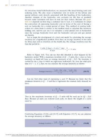
Refer to Figure 10.6. You can see that this situation is what happens in the
backorder model. With a maximum inventory of Q S units, the t 1 days we have
inventory on hand will have an average inventory of (Q S)/2. No inventory is
carried for the t 2 days in which we experience backorders. So, over the total cycle
time of T ¼ t 1 + t 2 days, we can calculate the average inventory as follows:

1 1
Average inventory ¼ = 2 ðQ SÞt 1 þ 0t 2 ¼ = 2 ðQ SÞt 1 (10:17)
t 1 þ t 2 T

Can we find other ways of expressing t 1 and T? Because we know that the
maximum inventory is Q S and that d represents the constant daily demand, we
have:

Q S
t 1 ¼ days (10:18)
d

That is, the maximum inventory of Q S units will be used up in (Q S)/d
days. Because Q units are ordered each cycle, we know the length of a cycle
must be:

Q
T ¼ days (10:19)
d

Combining Equations (10.18) and (10.19) with Equation (10.17), we can calculate
the average inventory as follows:

1 = 2 ðQ SÞ½ðQ SÞ=dŠ ðQ SÞ 2
Average inventory ¼ ¼ (10:20)
Q=d 2Q

Copyright 2014 Cengage Learning. All Rights Reserved. May not be copied, scanned, or duplicated, in whole or in part. Due to electronic rights, some third party content may be suppressed from the eBook and/or eChapter(s). Editorial review has
deemed that any suppressed content does not materially affect the overall learning experience. Cengage Learning reserves the right to remove additional content at any time if subsequent rights restrictions require it.