Page 437 -

ECONOMIC PRODUCTION LOT SIZE MODEL 417

To illustrate we shall use the following example. EnviroHealth, a large pharma-
ceutical company, manufactures a special type of anti-bacterial soap used in local
health clinics. The soap is sold in one litre bottles and because of the specialist
nature of the product and the strict hygiene controls that are enforced during
production, the soap is produced only at limited times and not continuously. The
company estimates that its current maximum annual production capacity is 60 000
litres. Current annual demand is 26 000 litres and is fairly constant through the year.
Given that the company will not be producing the product continuously through the
year it needs to know how often to produce the product and how much of the
product to produce each time.
For example, if we have a production system that produces 50 units per day and
we decide to schedule ten days of production, we have a 50(10) ¼ 500-unit produc-
tion lot size. The lot size is the number of units in an order. In general, if we let Q
indicate the production lot size, the approach to the inventory decisions is similar to
the EOQ model; that is, we build a holding and ordering cost model that expresses
the total cost as a function of the production lot size. Then we attempt to find the
production lot size that minimizes the total cost.
One other condition that should be mentioned at this time is that the model only
applies to situations where the production rate is greater than the demand rate; the
production system must be able to satisfy demand. For instance, if the constant
demand rate is 400 units per day, the production rate must be at least 400 units per
day to satisfy demand. For EnviroHealth, this requirement is satisfied: annual
production capacity is 60 000 litres whilst annual demand is only 26 000.
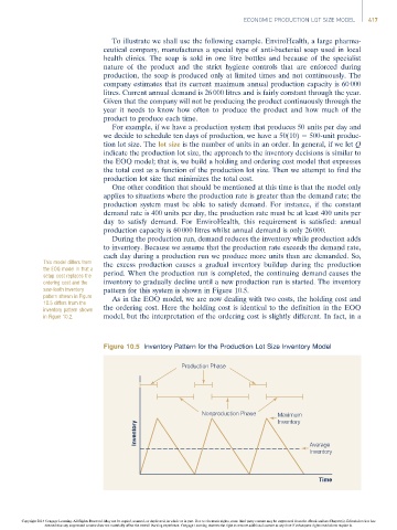
During the production run, demand reduces the inventory while production adds
to inventory. Because we assume that the production rate exceeds the demand rate,
each day during a production run we produce more units than are demanded. So,
This model differs from the excess production causes a gradual inventory buildup during the production
the EOQ model in that a
setup cost replaces the period. When the production run is completed, the continuing demand causes the
ordering cost and the inventory to gradually decline until a new production run is started. The inventory
saw-tooth inventory pattern for this system is shown in Figure 10.5.
pattern shown in Figure As in the EOQ model, we are now dealing with two costs, the holding cost and
10.5 differs from the
inventory pattern shown the ordering cost. Here the holding cost is identical to the definition in the EOQ
in Figure 10.2. model, but the interpretation of the ordering cost is slightly different. In fact, in a

Figure 10.5 Inventory Pattern for the Production Lot Size Inventory Model

Production Phase

Nonproduction Phase Maximum
Inventory
Inventory

Average
Inventory

Time

Copyright 2014 Cengage Learning. All Rights Reserved. May not be copied, scanned, or duplicated, in whole or in part. Due to electronic rights, some third party content may be suppressed from the eBook and/or eChapter(s). Editorial review has
deemed that any suppressed content does not materially affect the overall learning experience. Cengage Learning reserves the right to remove additional content at any time if subsequent rights restrictions require it.