Page 436 -

416 CHAPTER 10 INVENTORY MODELS

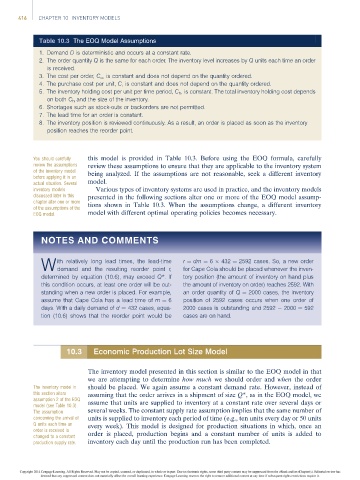
Table 10.3 The EOQ Model Assumptions
1. Demand D is deterministic and occurs at a constant rate.
2. The order quantity Q is the same for each order. The inventory level increases by Q units each time an order
is received.
3. The cost per order, C o , is constant and does not depend on the quantity ordered.
4. The purchase cost per unit, C, is constant and does not depend on the quantity ordered.
5. The inventory holding cost per unit per time period, C h , is constant. The total inventory holding cost depends
on both C h and the size of the inventory.
6. Shortages such as stock-outs or backorders are not permitted.
7. The lead time for an order is constant.
8. The inventory position is reviewed continuously. As a result, an order is placed as soon as the inventory
position reaches the reorder point.

You should carefully this model is provided in Table 10.3. Before using the EOQ formula, carefully
review the assumptions review these assumptions to ensure that they are applicable to the inventory system
of the inventory model
before applying it in an being analyzed. If the assumptions are not reasonable, seek a different inventory
actual situation. Several model.
inventory models Various types of inventory systems are used in practice, and the inventory models
discussed later in this presented in the following sections alter one or more of the EOQ model assump-
chapter alter one or more tions shown in Table 10.3. When the assumptions change, a different inventory
of the assumptions of the
EOQ model. model with different optimal operating policies becomes necessary.

NOTES AND COMMENTS

ith relatively long lead times, the lead-time r ¼ dm ¼ 6 432 ¼ 2592 cases. So, a new order
W demand and the resulting reorder point r, for Cape Cola should be placed whenever the inven-
determined by equation (10.6), may exceed Q*. If tory position (the amount of inventory on hand plus
this condition occurs, at least one order will be out- the amount of inventory on order) reaches 2592. With
standing when a new order is placed. For example, an order quantity of Q ¼ 2000 cases, the inventory
assume that Cape Cola has a lead time of m ¼ 6 position of 2592 cases occurs when one order of
days. With a daily demand of d ¼ 432 cases, equa- 2000 cases is outstanding and 2592 2000 ¼ 592
tion (10.6) shows that the reorder point would be cases are on hand.

10.3 Economic Production Lot Size Model

The inventory model presented in this section is similar to the EOQ model in that
we are attempting to determine how much we should order and when the order
The inventory model in should be placed. We again assume a constant demand rate. However, instead of
this section alters assuming that the order arrives in a shipment of size Q*, as in the EOQ model, we
assumption 2 of the EOQ
model (see Table 10.3). assume that units are supplied to inventory at a constant rate over several days or
The assumption several weeks. The constant supply rate assumption implies that the same number of
concerning the arrival of units is supplied to inventory each period of time (e.g., ten units every day or 50 units
Q units each time an every week). This model is designed for production situations in which, once an
order is received is
changed to a constant order is placed, production begins and a constant number of units is added to
production supply rate. inventory each day until the production run has been completed.

Copyright 2014 Cengage Learning. All Rights Reserved. May not be copied, scanned, or duplicated, in whole or in part. Due to electronic rights, some third party content may be suppressed from the eBook and/or eChapter(s). Editorial review has
deemed that any suppressed content does not materially affect the overall learning experience. Cengage Learning reserves the right to remove additional content at any time if subsequent rights restrictions require it.