Page 434 -

414 CHAPTER 10 INVENTORY MODELS

where
r ¼ reorder point
d ¼ demand per day
m ¼ lead time for a new order in days
The question of how frequently the order will be placed can now be answered.
The period between orders is referred to as the cycle time. Previously in equation
(10.2), we defined D/Q as the number of orders that will be placed in a year. Thus,
D/Q* ¼ 104 000/1824 ¼ 57 is the number of orders CBC will place for Cape Cola
each year. If CBC places 57 orders over 250 working days, it will order approx-
imately every 250/57 ¼ 4.39 working days. So, the cycle time is 4.39 working days.
3
The general expression for a cycle time of T days is given by:

250 250Q
T ¼ ¼ (10:7)
D=Q D

Sensitivity Analysis for the EOQ Model

Even though substantial time may have been spent in arriving at the cost per order
(E32) and the holding cost rate (25 per cent), we should realize that these figures
are at best good estimates. So, we may want to consider how much the recom-
mended order quantity would change with different estimated ordering and holding
costs. To determine the effects of various cost scenarios, we can calculate the
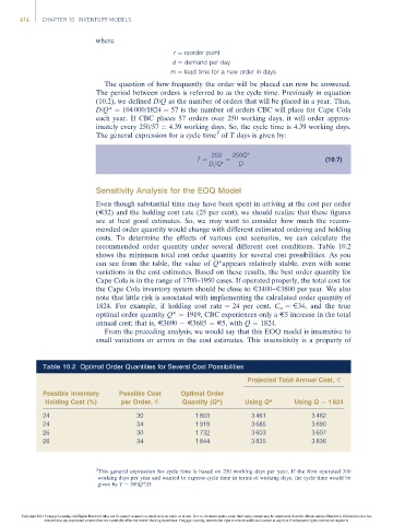
recommended order quantity under several different cost conditions. Table 10.2
shows the minimum total cost order quantity for several cost possibilities. As you
can see from the table, the value of Q*appears relatively stable, even with some
variations in the cost estimates. Based on these results, the best order quantity for
Cape Cola is in the range of 1700–1950 cases. If operated properly, the total cost for
the Cape Cola inventory system should be close to E3400–E3800 per year. We also
note that little risk is associated with implementing the calculated order quantity of
1824. For example, if holding cost rate ¼ 24 per cent, C o ¼ E34, and the true
optimal order quantity Q* ¼ 1919, CBC experiences only a E5 increase in the total
annual cost; that is, E3690 E3685 ¼ E5, with Q ¼ 1824.
From the preceding analysis, we would say that this EOQ model is insensitive to
small variations or errors in the cost estimates. This insensitivity is a property of

Table 10.2 Optimal Order Quantities for Several Cost Possibilities

Projected Total Annual Cost, E
Possible Inventory Possible Cost Optimal Order
Holding Cost (%) per Order, E Quantity (Q*) Using Q* Using Q ¼ 1 824

24 30 1 803 3 461 3 462
24 34 1 919 3 685 3 690
26 30 1 732 3 603 3 607
26 34 1 844 3 835 3 836

3
This general expression for cycle time is based on 250 working days per year. If the firm operated 300
working days per year and wanted to express cycle time in terms of working days, the cycle time would be
given by T ¼ 300Q*/D.

Copyright 2014 Cengage Learning. All Rights Reserved. May not be copied, scanned, or duplicated, in whole or in part. Due to electronic rights, some third party content may be suppressed from the eBook and/or eChapter(s). Editorial review has
deemed that any suppressed content does not materially affect the overall learning experience. Cengage Learning reserves the right to remove additional content at any time if subsequent rights restrictions require it.