Page 429 -

ECONOMIC ORDER QUANTITY (EOQ) MODEL 409

One of the most criticized Strictly speaking, these weekly demand figures do not show a constant demand rate.
assumptions of the EOQ However, given the relatively low variability exhibited by the weekly demand, inven-
model is the constant
demand rate. Obviously, tory planning with a constant demand rate of 2000 cases per week appears accept-
the model would be able. In practice, you will find that the actual inventory situation seldom, if ever,
inappropriate for items satisfies the assumptions of the model exactly. So, in any particular application, the
with widely fluctuating
and variable demand manager must determine whether the model assumptions are close enough to reality
rates. However, as this for the model to be useful. In this situation, because demand varies from a low of
example shows, the EOQ 1900 cases to a high of 2100 cases, the assumption of constant demand of 2000 cases
model can provide a per week appears to be a reasonable approximation.
realistic approximation of The how-much-to-order decision involves selecting an order quantity that draws a
the optimal order quantity
when demand is compromise between (1) keeping small inventories and ordering frequently, and (2)
relatively stable and keeping large inventories and ordering infrequently. The first alternative can result
occurs at a nearly in undesirably high ordering costs, while the second alternative can result in unde-
constant rate.
sirably high inventory holding costs. To find an optimal compromise between these
conflicting alternatives, let us consider a mathematical model that shows the total
As with other quantitative cost as the sum of the holding cost and the ordering cost. 1
models, accurate To estimate the holding cost of its inventory, CBC uses its cost of capital at an
estimates of cost annual rate of 18 per cent. Other holding costs incurred involve insurance, breakage
parameters are critical. In
the EOQ model, and pilfering and these are estimated at an additional 7 per cent of inventory. So, for
estimates of both the CBC, the total holding cost is 18% + 7% ¼ 25% of the value of the inventory. Each
inventory holding cost case of Cape Cola has a cost of E8 so the holding cost per year for each case is E2
and the ordering cost are (0.25 8).
needed. Also see
footnote 1, which refers The next step in the inventory analysis is to determine the ordering cost. For
to relevant costs. CBC, the largest portion of the ordering cost involves the salaries of the staff in
CBC’s purchasing department. An analysis of the purchasing process showed that a
purchaser spends approximately 45 minutes preparing and processing an order for
Cape Cola. With a wage rate and fringe benefit cost for purchasers of E20 per hour,
the labour portion of the ordering cost is E15. Making allowances for paper,
postage, telephone, transportation and receiving costs at E17 per order, the manager
estimates that the ordering cost is E32 per order. That is, CBC is paying E32 per
order regardless of the quantity requested in the order.
Most inventory cost The holding cost, ordering cost and demand information are the three data items
models use an annual that must be known prior to the use of the EOQ model. After developing these data
cost. Thus, demand
should be expressed in for the CBC problem, we can look at how they are used to develop a total cost
units per year and model. We begin by defining Q as the order quantity. So, the how-much-to-order
inventory holding cost decision involves finding the value of Q that will minimize the sum of holding and
should be based on an ordering costs.
annual rate.
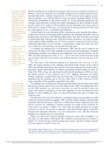
The inventory for Cape Cola will have a maximum value of Q units when an order
of size Q is received from the supplier. CBC will then satisfy customer demand from
inventory until the inventory is depleted, at which time another shipment of Q units
will be received. So, assuming a constant demand, the graph of the inventory for
Cape Cola is as shown in Figure 10.1. Note that the graph indicates an average
inventory of ½Q for the period in question. This level should appear reasonable
because the maximum inventory is Q, the minimum is zero, and the inventory
declines at a constant rate over the period.
Figure 10.1 shows the inventory pattern during one order cycle of length T.As
time goes on, this pattern will repeat. The complete inventory pattern is shown in
Figure 10.2. If the average inventory during each cycle is ½Q, the average inventory
over any number of cycles is also ½Q.

1
Even though analysts typically refer to ‘total cost’ models for inventory systems, often these models describe
only the total variable or total relevant costs for the decision being considered. Costs that are not affected by the
how-much-to-order decision are considered fixed or constant and are not included in the model.

Copyright 2014 Cengage Learning. All Rights Reserved. May not be copied, scanned, or duplicated, in whole or in part. Due to electronic rights, some third party content may be suppressed from the eBook and/or eChapter(s). Editorial review has
deemed that any suppressed content does not materially affect the overall learning experience. Cengage Learning reserves the right to remove additional content at any time if subsequent rights restrictions require it.