Page 354 - Applied Numerical Methods Using MATLAB

CONSTRAINED OPTIMIZATION 343

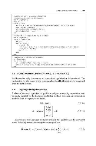
function chrms2 = crossover(chrms2,Nb)
% crossover between two chromosomes
Nbb = length(Nb);
b2=0;
for m = 1:Nbb
b1 = b2 + 1; bi = b1 + mod(floor(rand*Nb(m)),Nb(m)); b2 = b2 + Nb(m);
tmp = chrms2(1,bi:b2);
chrms2(1,bi:b2) = chrms2(2,bi:b2);
chrms2(2,bi:b2) = tmp;
end
function P = mutation(P,Nb,Pm) % mutation
Nbb = length(Nb);
for n = 1:size(P,1)
b2=0;
for m = 1:Nbb
if rand < Pm
b1 = b2 + 1; bi = b1 + mod(floor(rand*Nb(m)),Nb(m)); b2 = b2 + Nb(m);
P(n,bi) = ~P(n,bi);
end
end
end
function is = shuffle(is) % shuffle
N = length(is);
for n = N:-1:2
in = ceil(rand*(n - 1)); tmp = is(in);
is(in) = is(n); is(n) = tmp; %swap the n-th element with the in-th one
end

7.2 CONSTRAINED OPTIMIZATION [L-2, CHAPTER 10]
In this section, only the concept of constrained optimization is introduced. The
explanation for the usage of the corresponding MATLAB routines is postponed
until the next section.

7.2.1 Lagrange Multiplier Method
A class of common optimization problems subject to equality constraints may
be nicely handled by the Lagrange multiplier method. Consider an optimization
problem with M equality constraints.
Min f(x) (7.2.1a)
 
h 1 (x)
 h 2 (x) 
s.t. h(x) =   = 0 (7.2.1b)
:
 
h M (x)
According to the Lagrange multiplier method, this problem can be converted
to the following unconstrained optimization problem:

M
T
Min l(x, λ) = f(x) + λ h(x) = f(x) + λ m h m (x) (7.2.2)
m=1