Page 357 - Applied Numerical Methods Using MATLAB

346 OPTIMIZATION
2
f(x) = x 1 + x 2 = 2

f(x) = x 1 + x 2
5
2
2
0 h(x) = x 1 + x 2 −2 = 0
0 2 2
h(x) = x 1 + x 2 −2 = 0
−5
−2
2
0 f(x) = x 1 + x 2 = −2
0
−2
−2 −2 −2 0 2
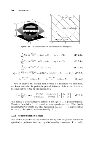
Figure 7.11 The objective function with constraint for Example 7.2.

∂ (7.2.3a)
l(x,λ) = 1 + 2λx 1 = 0, x 1 =−1/2λ (E7.2.4a)
∂x 1
∂ (7.2.3a)
l(x,λ) = 1 + 2λx 2 = 0, x 2 =−1/2λ (E7.2.4b)
∂x 2
∂ (7.2.3b) 2 2
l(x,λ) = x + x − 2 = 0 (E7.2.4c)
1
2
∂λ
2
2
2
x + x 2 (E7.2.4c) 2 (E7.2.4a,b) (−1/2λ) + (−1/2λ) = 2, λ =±1/2 (E7.2.5)
→
=
1 2
(E7.2.4a) (E7.2.4b)
x 1 = −1/2λ =∓1, x 2 = −1/2λ =∓1 (E7.2.6)
Now, in order to tell whether each of these is a minimum or a maximum,
we should determine the positive/negative-definiteness of the second derivative
(Hessian matrix) of l(x, λ) with respect to x.
2
2
∂ 2 ∂ l/∂x 2 ∂ l/∂x 1 ∂x 2 2λ 0
H = l(x, λ) = 2 1 2 2 = (E7.2.7)
∂x 2 ∂ l/∂x 2 ∂x 1 ∂ l/∂x 2 0 2λ
This matrix is positive/negative-definite if the sign of λ is positive/negative.
Therefore, the solution (x 1 ,x 2 ) = (−1, −1) corresponding to λ = 1/2is a (local)
minimum that we want to get, while the solution (x 1 ,x 2 ) = (1, 1) corresponding
to λ =−1/2 is a (local) maximum (see Fig. 7.11).

7.2.2 Penalty Function Method
This method is practically very useful for dealing with the general constrained
optimization problems involving equality/inequality constraints. It is really