Page 361 - Applied Numerical Methods Using MATLAB

350 OPTIMIZATION
minimum, which is on the intersection of the two boundary curves corresponding
to the fourth and fifth constraints of (E7.3.1b).

7.3 MATLAB BUILT-IN ROUTINES FOR OPTIMIZATION

In this section, we apply several MATLAB built-in unconstrained optimization rou-
tines including “fminsearch()”and “fminunc()” to the same problem, expecting
that their nuances will be clarified. Our intention is not to compare or evaluate the
performances of these sophisticated routines, but rather to give the readers some
feelings for their functional differences. We also introduce the routine “linprog()”
implementing Linear Programming (LP) scheme and “fmincon()” designed for
attacking the (most challenging) constrained optimization problems. Interested
readers are encouraged to run the tutorial routines “optdemo”or “tutdemo”, which
demonstrate the usages and performances of the representative built-in optimiza-
tion routines such as “fminunc()”and “fmincon()”.

7.3.1 Unconstrained Optimization
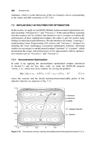
In order to try applying the unconstrained optimization routines introduced
in Section 7.1 and see how they work, we made the MATLAB program
“nm731_1.m”, which uses those routines for solving the problem
2
2
2
Min f(x) = (x 1 − 0.5) (x 1 + 1) + (x 2 + 1) (x 2 − 1) 2 (7.3.1)
where the contours and the (local) maximum/minimum/saddle points of this
objective function are depicted in Fig. 7.13.

1.5

1
minimum
maximum
0.5 saddle

0
steepest descent
−0.5
Newton

−1

−1.5
−1.5 −1 −0.5 0 0.5 1
Figure 7.13 The contours, minima, maxima, and saddle points of the objective function (7.3.1).